Deep Learning - Neural Networks
Neural Networks
Neural networks are simply function compositions.
- Feedforward networks
$$ y = f(g(x, \theta_g), \theta_f) $$
- Recurrent networks
$$ y_t = f(y_{t-1}, x_t, \theta) $$
Generally, you can think of neural networks as function approximation machines, where we want to find appropriate $\theta$ to make $f^{*}$ as similar as possible to the true function $f$.
In practice, there are lots of things to consider when designing a neural network. Basically, we need to consider the following factors,
- Loss function
- Architecture of the network
- How many layers?
- How many units in each layer?
- How are these layers connected?
- Optimisation Algorithm
Loss Function
In classification tasks, target variables are categorical, so we need to find a method to transform them into numerical values. Typically, we use one-hot encoding to encode each category into a binary value. If an example belongs to class $j$, then the true target value is $C_j = 1$, otherwise $C_j = 0$. When we make predictions, we’d like to predict the probability of an example belonging to a class. For example, we may have such a prediction $(0.1,0.7,0.2)$. Since class 2 has the highest probability, we say that this example is classified as class 2.
But how to quantify the difference between predictions and the ground truth so as to find the best parameters? In Machine Learning, we have learned mean squared error (MSE) and cross-entropy as the loss functions. So, which one to use?
MSE
Let’s take the derivative of MSE w.r.t $w$. The equation below shows that the gradient of MSE w.r.t $w$ is the product of the difference between the target value $y$ and predicted value $\sigma(z)$ and the gradient of the activation function.
$$ \frac {\partial }{\partial w}\frac{1}{2}(y - \sigma(z))^2 = (y - \sigma(z))\sigma'(z)x $$
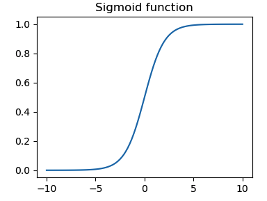
A widely used activation function in binary classification is the sigmoid function. From Figure 1, we see that when the predicted value is close to 1/0, the curve gets very flat, indicating $\sigma'(z)$ becomes very small. If the ground truth is opposite to the predicted value, our machine will learn slowly as the gradient of MSE w.r.t. $w$ is small.
Cross-Entropy
Entropy is an important concept in information theory. Basically, it tells us the average information a random variable conveys. Cross-entropy measures the difference between two distributions, where $f(x)$ is considered as the ground truth. Thus, a smaller cross-entropy indicates better learning.
$$ E = -\sum_{x \in X} f(x) \text{log} g(x) $$
Does it have the problem of slow learning? Let’s take the derivative of $E$ w.r.t $w_j$ (suppose it’s binary classification)
$$ \frac{\partial L}{\partial w_j} = - \frac{1}{n} \sum_x (\frac{y}{\sigma(z)} - \frac{1 - y}{1 - \sigma(z)})\sigma'(z)x_j = - \frac{1}{n} \sum_x (\sigma(z) - y) x_j $$
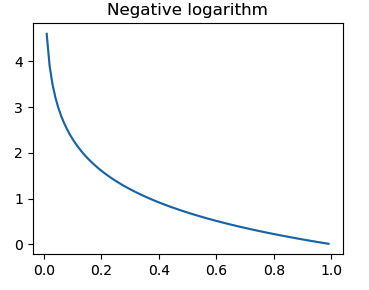
We see that the gradient of $w_j$ is determined by the error in the output. In other words, cross-entropy punishes the wrong classification heavily. Figure 2 also shows that misclassified point conveys much information.
Activation Function
Why
Why do we need an activation function?
Deep learning works by mimicking how a human brain learns. Every second, our brains receive a lot of information, but not all of them are useful. Some information will be ignored, otherwise our brains will be overloaded. In deep learning, we need to find a method to do the same thing. Activation functions, as their name suggests, decide whether to fire neurons or not.
On the other hand, since neural networks are composed of multiple layers and each layer can be expressed as $Y = XW$, the final output is given as $ y = XW_1 W_2..W_n = XW$, where $W = W_1W_2…W_n$. If all functions are linear, there is no need to add the depth of the network as we can just use a single layer to achieve this. To capture the features, we must use a nonlinear function, also known as an activation function, which is applied to each hidden unit following an affine transformation controlled by parameters.
What
So, what should a valid activation function look like?
- differentiable
- because deep learning is gradient-based learning, we need to know in which direction and how much to move in the parameter space
- monotonic
Binary Step function
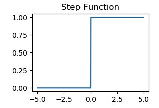
A simple way to fire a neuron is to set a threshold. If the output of a neuron is greater than zero, the step function will return 1 and this neuron will be activated, otherwise it will be deactivated.
- Equation
def step(x):
    if x > 0:
        return 1
    return 0
- Range: $\{0, 1\}$
- Pros
- simple
- Cons
- only suitable for binary classificaition
- the gradient is zero, so the parameters will not updated via backprop
Identity
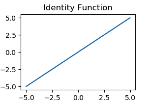
Identity function is a linear function that returns the multiple of the input.
- Equation
$$ f(x) = ax $$
-
Range: $(-\infin, \infin)$
-
Pros
- The gradient is non-zero
-
Cons
- However, the gradient is a constant value that does not depend on the inputs, so learning will not be improved from errors since the gradient is always the same.
Sigmoid
- Equation
$$ f(z) = \frac{1}{1 + e^{-z}} $$
- Range: $[0, 1]$
- Pros
- Smooth S-shaped and continuously differentiable
- It is suitable for predicting the probability as an output
- Cons
- The gradient is small as $z$ is far away from 0, which will cause ‘vanishing gradient’

x = torch.arange(-5, 5, 0.1)
# F.sigmoid is deprecated
y = torch.sigmoid(x)
Tanh
- Equation
$$ f(x) = \text{tanh} (x) = \frac{2}{1+e^{-2x}} - 1 $$
-
Range: $[-1, 1]$
-
Pros
- Similar to sigmoid, but it’s symmetric around 0
- The gradient is steeper than sigmoid
-
Cons
- vanishing gradient

x = torch.arange(-5, 5, 0.1)
# F.tanh is deprecated
y = torch.tanh(x)
ReLU
- Equation
$$ f(x) = \text{max} (0, x) $$
-
Range: $[0, \infin)$
-
Pros
- sparse network and efficient
- simpler mathematical operation
-
Cons
- dying reLU, since neurons with negative values will be deactivated, and thus the weights for them will not be updated due to the zero gradient
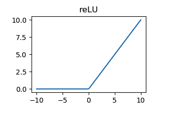
x = torch.arange(-5, 5, 0.1)
y = F.relu(x)
Leaky ReLU
A solution to solve dying ReLU problem is to make the horizontal line into non-horizaontal line. The leak coefficient that controls the slope, also known negative_slope in PyTorch, is a learned parameter, typically, it’s $0.01$.
$$ f(x) = \text{max} (0, x) + \text{negative\_slope} * \text{min}(0, x) $$
x = torch.arange(-5, 5, 0.1)
y = F.leaky_relu(x)
Parametric ReLU
$$ f(x) = \text{max} (0, x) + \text{a} * \text{min}(0, x) $$
x = torch.arange(-5, 5, 0.1)
# weight must be a tensor
y = F.prelu(x, torch.tensor(0.25))