Deep Learning - CNN
Convolutional Neural Networks (CNN) are widely used for image classification, object detection and other tasks related to images or videos in the field of computer vision. Plenty of architectures based on convolution operation have been proposed in recent years, such as AlexNet and ResNet. So, how do CNNs work? Why not use MLP? In this post, we will go through the fundamentals of CNN and several ConvNets to develop a big picture of CNN.
Convolution
Convolution Operation
As its name suggests, CNN employes a special mathematical operation called convolution rather than matrix multiplication in the networks. So, what’s the convolution? Mathematically, the convolution operation is defined as
$$ s(t) = (x \ast w)(t) = \int x(a) w(t - a)da $$ where $x$ is the real valued function of $t$, $w$ is a weighting function that measures the weight of $x$ at the point of $t$. So, convolution is a weighted average operation. For example, $x$ returns the real-time position of a plane, but the returned positions have some noises. A solution is to average the positions of recent moments. Obviously, the most recent moment has the highest weight. For functions that return discrete values, the discrete convolution operation is defined as
$$ s(t) = (x \ast w)(t) = \sum_{a = -\infin}^{\infin} x(a) w(t - a) $$
Cross-correlation
The above equation considers only one variable. However, in machine learning, we often deal with multi-dimensional data. In this case, the convolution is simply the sum of the products from all dimensions,
$$ S(i, j) = (I \ast K)(i, j) = \sum_{m}\sum_{n} I(m, n)K(i - m, j - n) $$
where $I$ is a two-dimensional input array, and $K$ is a two-dimensional weighting matrix, also known as a kernel. Careful people will notice that $K$ is flipped when multiplying $I$. Suppose $I$ represents an image whose width is $m$ and height is $n$, as $m$ increases, the index of $I$ increases while the index of $K$ decreases. That is, the left part of the image multiplies the right part of the kernel.
In deep learning, flipping a kernel or not is unnecessary, since the kernel is obtained through learning. If it should be flipped, then the learned kernel is flipped. Thus, there is no need to explicitly specify a flipped kernel, let alone we do not know what it is exactly. In fact, many deep learning frameworks implement a similar function and call it as convolution. This function is cross-correlation, which is the same as convolution but without flippling
$$ S(i, j) = (I \ast K)(i, j) = \sum_{m}\sum_{n} I(i+m, j+n)K(m, n) $$ In CNN, $I$ and $K$ are often referred to as the input and the kernel, respectively. The output is often referred to as the feature map.
Receptive Field
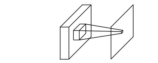
In CNN, the scalar obtained from the cross correlation is referred to a neuron. The area enclosed by relevant inputs is called the receptive field of that neuron. So, convolution is simply an element-wise multiplication of learned weights (kernel) across a receptive field, which is repeated at various positions across the input. Normally, we also add a bias term for each filter.
Why CNN
Okay, but we still do not know why to use CNN instead?
Sparse connectivity
In MLP, all input variables are connected to a hidden neuron. Suppose there are $m$ features and $h$ hidden units, we have $m * h$ parameters to learn. If we restrict the number of connections, say $k$, then there are only $k * h$ parameters. Generally, $k$ is far smaller than $m$, which greatly improves the efficiency of learning. This technique can be easily achieved in CNN through a kernel whose size is smaller than the input. So, sparse connectivity in CNN means
- reduce memory space to store the parameters
- reduce the number of computation operations
- increase the efficiency of learning
Parameter sharing
Another difference is that kernels in CNN are shared. Instead of different $k$ parameters for each hidden neuron in the traditional neural networks, there are only $k$ shared parameters for each element in each feature map (for now, we only consider one channel).
Translation equivariance
Translation equivariance indicates that CNN should get the same result from the same pattern, no matter where the pattern is. Mathematically, it can be expressed as,
$$ I(T(x)) = T(I(x)) $$ where $T$ represents a transformation function, and $I$ is the mapping function. If the object of interest in the inputs moves, the corresponding representation should move the same amount in the feature map due to parameter sharing.
This works based on assumption that we want to detect a specific pattern in an image, irrelevant to locations. Suppose there are two of the same cats but in different positions in an image, it is redundant to learn the same parameters to classify them as cats. As a human, we know the second one is also a cat, because we see that it has whiskers, furs, ears, tails and other characters of being a cat. Thus, we hope the kernels or convolutions will also be able to extract these features, regardless of positions. As long as an area contains these features, it will be classified as cats.
Padding and Stride
Now let’s see how a kernel really works. Figure 2 depicts the convolution operation between a two-dimensional array and a kernel with the size of $2 \times 2$ .
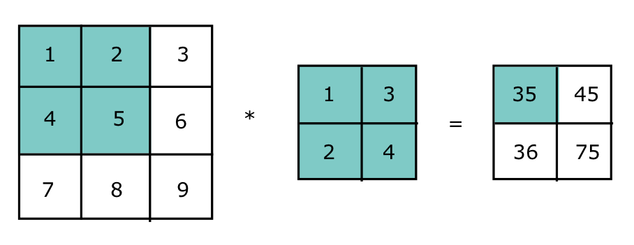
The output tensor is derived as follows
$$ 1 * 1 + 2 * 3 + 4 * 2 + 5 * 4 = 35 \\ 2 * 1 + 3 * 3 + 5 * 2 + 6 * 4 = 45 \\ 4 * 1 + 5 * 3 + 7 * 2 + 8 * 4 = 36 \\ 5 * 1 + 6 * 3 + 8 * 2 + 9 * 4 = 75 $$
We also noticed that the size of the output tensor is $2 \times 2$, which is smaller than the input size ($3 \times 3$). In fact, the output size is determined by the shape of the input and kernel, as shown below
$$ ( I_h - K_h + 1 ) \times ( I_w - K_w + 1 ) $$
where $I$ is the input size, and $K$ is the size of the kernel. In this example, the output size is $ (3 - 2 + 1) \times ( 3 - 2 + 1) = 2 \times 2 $.
Why padding
Padding and stride are two commonly used techniques in CNN. But why?
If we further apply another kernel to the output, we will get a scalar in the end, which is not always the desired result. Sometimes we want to preserve the shape of the input. So, we often use zero-padding to retain the size.
Besides, each time we perform convolution operation, we will lose pixels on the boundaries of the image as we only scan the border only once. In the above example, we can see that pixels on the top and bottom border of the image ($1, 3, 7, 9$) appear only once in the convolution operation, while the inner part of the image (2,4,5,6,8) present twice.
Why stride
On the other hand, the step that the kernel moves each time either horizontally or vertically is 1, which is expensive. Sometimes we might want to quickly obtain a reduced output, a solution is to increase step.
With padding and stride, the output shape is given as
$$ \lfloor (I_h + P_h - K_h) / S_h + 1 \rfloor \times \lfloor (I_w + P_w - K_w) / S_w + 1 \rfloor $$
where $P$ and $S$ indicates the padding and stride, respectively. From the above equation, we can see that
- the output size increases as $P_h$ and $P_w$ increases when $S$ stays the same
- if $P_h = K_h - S_h$ and $P_w = K_w - S_h$, the shape of output is $I_h/S_h \times I_w / S_w$
- if $S_h = 1$ and $S_w = 1$
- an odd value of $K_h$ will pad the same rows in both sides of the height;
- an even value of $K_h$, well, one solution is to pad $\lfloor P_h/2 \rfloor$ rows on the top of the image and $\lceil P_h/2 \rceil$ rows on the bottom
That’s why you often see odd kernels in CNN (stride is 1 by default). Besides, in practice, we often set $P_h = P_w$ and $S_h = S_w$.
Multiple Channels
So far, we only considered a single-layer input. As we know, an image has three channels —— R, G, B. That is, we need to perform convolution at each channel and then add the respective feature map together to obtain the final output, which is depicted in Figure 3.

Figure 3 shows that the number of kernels are the same as the number of channels in the input data. To make a clear distinction between one kernel and multiple kernels, we note that a kernel is a two-dimensional array (a slice of a filter) while a set of kernels are called a filter. In fact, many articles use them interchangeably. So far so good. But we still get one output. How do we get multiple outputs? —— The answer is to use multiple filters.
Now let’s focus on the number of parameters. Let $C_I$ and $C_O$ be the number of input and output channels, and $K_w$ and $K_h$ be the width and height of each kernel, the total number of parameter needed in convolution layer is given as (bias is ignored)
$$ C_O * C_I * K_w * K_w $$
In summary, the core parameters of a convolution layer are
- the dimensionality of the input
- the spatial extent of the kernel
- the number of kernels ( output channels )
Data Types
Convolution can be applied to many dimensionalities and types of data, for example
| Single Channel | Multiple Channels | |
|---|---|---|
| 1D | Audio | multiple sensor data over time |
| 2D | greyscale images | Colour image data |
| 3D | Volumetric data | Colour Video Data |
1 x 1 Kernel
The minimum size of a kernel is $1 \times 1$. It seems meaningless at first, since such a kernel does not correlate neighbouring pixels (capture local spatial information). Well, perhaps the only reason we’d like to use it is to change the dimension of the input channel ( the number of feature maps ).
$1 \times 1$ kernel will map each input element, so the output size is the same as the size of the input. However, the number of feature map depends on the number of filters we apply.
Pooling
A typical CNN contains three layers
- convolution layer
- activation layer
- pooling layer
Max/Avg Pooling
We have introduced the previous two layers, so what does pooling do? Pooling acts more like a window, where it reports some statistics from a group of data enclosed by that window, such as the maximum value or the average value, as shown in Figure 4 and Figure 5.
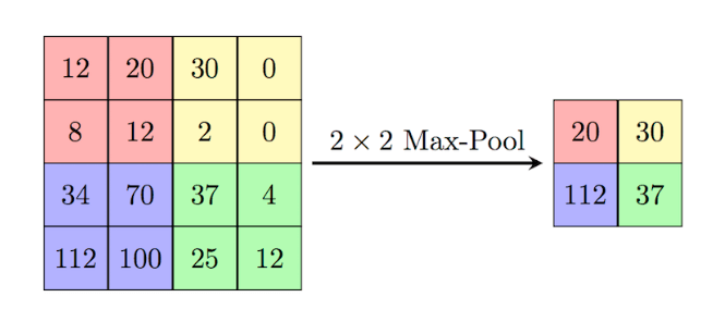
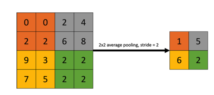
Unlike kernels, the pooling layer does not contain any parameter. But, why Pooling?
- decrease output dimension
- reduce memory space for storing parameters
- improve computational efficiency
- make feature representation approximately invariant to small translations of the input
In all cases, pooling helps to make the representation approximately invariant to small translations of the input. Invariance to translation means that if we translate the input by a small amount, the values of most of the pooled outputs do not change.
— Deep Learning, P336
Local VS Global Pooling
The above pooling operations are local pooling, because they result in a smaller feature map. On the contrary, global pooling reduces a feature map to a scalar, which often used near the end of networks to flatten feature mapts into a feature vector that can be fed into a MLP.
ConvNet
LeNet
LeNet was the earliest CNN proposed for handwritten digit recognition in 1998. As the oldest CNN architecture, it is a good starting point to learn how CNNs work before we move on to more complex networks.
Architecture

Figure 6 shows that LeNet has 7 layers consisting of
- 3 convolutional layers
- 2 sub-sampling layers
- 2 fully-connected layers
which are denoted by $C_x$, $S_x$, and $F_x$, respectively. Based on the formulas discussed above, we can derive the shape of the intermediate ouputs and learning parameters in each layer in LeNet, which is shown below.
| Layer | Kernel/Padding/Pooling | Output | Num of Paramaters |
|---|---|---|---|
| 1@32$\times$32 | |||
| C1 | 6@5 $\times$ 5, 0,1 | 6@28$\times$28 | 5*5*1*6+6 = 156 |
| S2 | 2$\times$2,0,2 | 6@14$\times$14 | 6*2=12 |
| C3 | 16@5 $\times$ 5,0,1 | 16@10$\times$10 | (5*5*3*6 + 6) + (5*5*4*9 + 9)+(5*5*6*1 + 1) =1516 |
| S4 | 2$\times$2, 0, 2 | 16@5$\times$5 | 16*2=32 |
| C5 | 120@5 $\times$ 5 | 120 | 5*5*16*120 + 120 = 48120 |
| F6 | NaN | 84 | 120*84+84 = 10164 |
| Output | NaN | 10 | 84 * 10 + 10 = 850 |
| 60,850 |
Table 1: The shape of the output and learning parameters in LeNet.
LeNet differs from modern CNNs in several ways
- the activation function is sigmoid function rather than reLU
- LeNet used subsampling (similar to average pooling) to reduce output dimentionality while modern CNNs use max pooling
Implementation
class LeNet(nn.Module):
    def __init__(self, num_class):
        super(LeNet, self).__init__()

        # in_channel, output_channel, kernel_size, stride, padding
        self.conv1 = nn.Conv2d(1,6,5)
        self.conv2 = nn.Conv2d(6,16,5)

        # self.conv3 = nn.Conv2d(16, 120, 5)
        self.fc1 = nn.Linear(16 * 5 * 5, 120)

        self.fc2 = nn.Linear(120, 84)
        self.fc3 = nn.Linear(84, num_class)

    def forward(self, x):
        x = F.sigmoid(self.conv1(x))
        x = F.avg_pool2d(x, 2)

        x = F.sigmoid(self.conv2(x))
        x = F.avg_pool2d(x, 2)

        x = torch.flatten(x, 1)
        x = F.sigmoid(self.fc1(x))
        x = F.sigmoid(self.fc2(x))
        logits = self.fc3(x)

        probs = F.softmax(logits, dim=1)

        return logits, probs
AlexNet
ImageNet is a publicly large image database for computer vision and deep learning research. The ImageNet Large Scale Visual Recognition Challenge (ILSVRC) was an annual image classification competition held from 2010 to 2017 using 1.3 million images in 1000 classes from the ImageNet dataset. AlexNet was the winner of ILSVRC 2012, achieving a top-5 error rate of 15.3%.
Architecture
](/blog/post/images/AlexNet.png#full)
As shown in Figure 7, AlexNet consists of 8 layers
- 5 convolutional layers
- 3 fully connected layers
Each layer and the corresponding number of learning parameters are shown below,
| Layer | Kernel/Padding/Pooling | Output | Num of Paramaters |
|---|---|---|---|
| 3@227$\times$227 | |||
| C1 | 96@11 $\times$11, 0, 4 | 96@55$\times$55 (=(227-11)/4+1) | 11*11*3*96+96 = |
| P2 | 3$\times$3, 0, 2 | 96@27$\times$27 (=(55-3)/2+1) | 0 |
| C3 | 256@5 $\times$ 5,2,1 | 256@27$\times$27 (=(27-5+2*2)/1 + 1) | 5*5*96*256 + 256 = |
| P4 | 3$\times$3, 0, 2 | 256@13$\times$13 (=(27-3)/2+1) | 0 |
| C5 | 384@3 $\times$ 3, 1, 1 | 384@13$\times$13 (=(13-3+1*2)/1+1) | 3*3*256*384 + 384 = |
| C6 | 384@3 $\times$ 3, 1, 1 | 384@13$\times$13 (=(13-3+1*2)/1+1) | 3*3*384*384 + 384 = |
| C7 | 256@3 $\times$ 3, 1, 1 | 256@13$\times$13 (=(13-3+1*2)/1+1) | 3*3*384*256 + 256 = |
| P8 | 3$\times$3, 0, 2 | 256@6$\times$6 (=(13-3)/2+1) | 0 |
| F9 | NaN | 4096 | 6*6*256*4096 + 4096 |
| F10 | NaN | 4096 | 4096*4096 +4096 |
| Output | NaN | 1000 | 4096*1000 + 1000 |
| 62,378,344 |
Table 1: The shape of the output and learning parameters in LeNet.
The main differences with LeNet includes
- reLU is used as the activation function
- overlapping max pooling is used to downsample the output
- GPU optimization
Avoid overfitting
- Data Augmentation
- Dropout
Implementation
VGG
VGG is short for Visual Geometry Group, which aimed to investigate the effect of convolutional network depth on large-scale image recognition. They increased the depth of network by using a small filter (3 $\times$ 3) instead of 5 $\times$ 5 or 7 $\times$ 7, showing significant improvements by adding the depth to 16-19. Typically, when we speak of VGG, we are talking about VGG-16 or VGG-19. The complete experimental ConvNet configurations are shown in Figure 8.
Architecture

The major difference to the previous networks is that the authors employed a stack of 3 $\times$ 3 filters to have receptive fields of 5 $\times$ 5, 7 $\times$ 7 or 11 $\times$ 11 rather than using larger filters that were the same size as the receptive fields. So, there are two questions,
- How it works?
- Why do we use it this way?
Figure 9 shows that we can use two 3 $\times$ 3 filters instead of a 5 $\times$ 5 filter to have the same receptive field. Similarly, three such filters will have a 7 × 7 effective receptive field.

What do we gain from the smaller filters?
- more non-linear activations
- each filter is followed by a non-linear activation function, which makes the decision function more discriminative
- decrease the number of parameters
- suppose both the input and output have $C$ channels, a single 5 $\times$ 5 filter has $5*5*C^2= 25C^2$ while the stacked two 3$\times$3 filters has $2*3*3*C^2=18C^2$
Drawbacks
Though VGG outperfoms other networks in ILSVRC, it’s difficult to train VGG from scratch because of
- long traning time
- huge number of weights
- much deeper network depth
- more fully-connected layers
ResNet
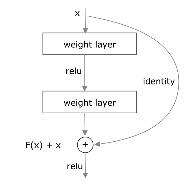
ResNet, short for Residual Network, was the winner of the ILSVRC 2015 classification challenge. Like VGG, there are many variants of ResNet, such as ResNet-18, ResNet-34, ResNet-50 and so on. Similar to other ConvNets, ResNet also has Conv layer, pooling, activation and FC layers. The difference is that ResNet introduced the identity connection, which is shown in Figure 10.
Motivation
In my opinion, the main idea of ResNet is similar to gradient boosting. We know that the idea of gradient boosting is to learn residuals. Similarly, ResNet tries to learn the residual function rather than the mapping function directly. What does this mean? First, neural networks are function approximators. Normally, we build a neural network to learn a specific function, say $h(x)$. Now, we suppose that $h(x)$ can be decomposed into two parts
$$ f(x) + x = h(x) $$
From Figure 10, we see that $f(x)$ is the target function that we want to learn while $x$ is the identity connection, If the output is $x$ ($h(x) =x$), then $f(x) = 0$. In other words, as learning progresses, $f(x)$ should approach $0$. That’s why $f(x)$ is called the residual function.
The effect of Identity Connection
VGG has demenstrated that as the depth of networks increases, the generalisation becomes better. However, the gradients are prone to shrink to zero if the network is too deep due to the chain rule, so some weights are never updated during learning. This is known as vanishing gradients. With ResNet, gradients can flow directly through the identity connection to the previous layers because of the addition operation, even if the graident in the residual block is very small.
Architecture
![Figure 11: ResNet 34 from original paper[Deep Residual Learning for Image Recognition]](/blog/post/images/resnet.png)

One problem is that $f(x)$ might have different shape with $x$. In this case, we employ 1 $\times$ 1 kernel to change the input shape, which is depicted by the dotted line in Figure 11. Mathematically, it can be expressed as
$$ f(x) + Wx = h(x) $$
References
- CNN Explainer
- Chapeter 9 Convolutional Networks - Deep Learning
- Simple Introduction to Convolutional Neural Networks
- A Gentle Introduction to 1×1 Convolutions to Manage Model Complexity
- An Intuitive Explanation of Convolutional Neural Networks
- CNNs and Equivariance
- Translation Invariance in Convolutional Neural Networks
- Understanding AlexNet
- VGG-16 Architecture: A Complete Guide
- Understading and visualizing ResNets
- ResNets
- K. He, X. Zhang, S. Ren and J. Sun, “Deep Residual Learning for Image Recognition,” in CVPR, 2016. https://arxiv.org/abs/1512.03385