Deep Learning - Preliminary
So far, we’ve covered most of the things that we should know about machine learning, including concepts, optimization, and popular models under the hood. Yet, some advanced techniques, such as the Gaussian Process and MCMC, are not mentioned. We will talk about them later. From now on, we will move to Deep Learning. But before that, we are going to revisit some math knowledge.
Linear Algebra
Tensor
We introduced tensors in the previous article. A tensor is a n-dimensional array of numbers.
- If $n=0$, it’s a scalar <=> a number mathmatically
- If $n =1$, it’s a vector <=> a list of numbers
- If $n=2$, it’s a matrix <=> a 2-dimensional array with two axises
- If $n>2$, it’s a tensor <=> an array with more than two axises
In linear algebra, we can add vectors, multiply a vector by a scalar, or do both of them.
Vector Addition
$$ \bold v=\begin{bmatrix}v_1\\ v_2\end{bmatrix} \bold w=\begin{bmatrix}w_1\\ w_2\end{bmatrix} \bold v+\bold w=\begin{bmatrix}v_1+w_1\\ v_2+w_2\end{bmatrix} $$
Scalar multiplication
$$ a \bold v=\begin{bmatrix}av_1\\ av_2\end{bmatrix} $$
Linear Combination
$$ c\bold v + d\bold w $$
Unit Vector
Vectors have both directions and length. The length is defined as follows,
$$ || \bold v|| = \sqrt{\bold v^T\bold v} $$ The vector whose length equals one is known as the unit vector,
$$ \bold v^T \bold v = 1 $$
Here are some unit vectors,
$$ \bold i=\begin{bmatrix}1\\ 0\end{bmatrix} \bold j=\begin{bmatrix}0\\ 1\end{bmatrix} \bold u=\begin{bmatrix}cos\theta\\ sin\theta\end{bmatrix} $$
A vector can be transformed into a unit vector by dividing it by its length, as shown below.
$$ \bold u = \frac{\bold v}{ || \bold v ||} $$
Dot product
$$ <v, w> = v \cdot w = v^Tw = v_1 * w_1 + v_2 * w_2 + … + v_n * w_n $$
- The order of $v$ and $w$ makes no difference.
- $v \cdot w$ is zero when $v$ and $w$ are prependicular.
For any real matrix 𝐴 and any vectors 𝐱 and 𝐲 , we have
$$ ⟨𝐴𝐱,𝐲⟩=⟨𝐱,𝐴^T𝐲⟩ $$
Ax = b
Mathematically, machine learning is all about $\bold A \bold x= \bold b$, where $A, b$ are known, and $x$ is unknown. We can interpret $Ax=b$ from two aspects
- $\bold A \bold x$ is a linear combination of the columns of A ( column picture )
- The system has solution only if the target $b$ lies in the column space of $A$
- $\bold A \bold x$ is dot products ( row picture )
- $m$ equations
Rank
To solve $x$ or to solve $m$ equations, we need $m$ pivots ($\bold A$ is an $m \times n$ matrix). Pivots are the diagnoal elements of $\bold A$. To find the pivots, we transform $A$ to an upper triangle matrix. Besides, we define the number of pivots of $A$ as the rank. In fact, rank contains the following meanings:
- the number of pivots
- $r$ independent rows or columns
- $r$ is the dimension of the column space or row space
However, it is not always lucky to obtain $m$ non-zero pivots. The possible solution could be either of the following cases
- no solution
$$ x - 2y = 1 \\ 0y = 8 $$
- infinitely many solutions
$$ x - 2y = 1 \\ 0y = 0 $$
- exactly one solution
$$ 3x - 2y = 5 \\ 2y = 4 $$
$\bold A$ in case 1 and 2 is called singular —— there is no second pivot.
- Singular equations have no solution or infinitely many solutions.
- Pivots must be non-zero becaue we have to divide by them.
Inverse Matrix
It is also possible to multiply the inverse of $\bold A$ to obtain $\bold x$ directly (closed-form solution), as shown below. $$ x = A^{-1}b $$ However, $A^{-1}$ is not always exist.
Is A invertible?
- $A$ must have $m$ non-zero pivots
- $A$ has $m$ linearly independent columns
- $det A \neq 0$
If $A$ is invertible,
-
the only solution to $Ax=b$ is $x=A^{-1}b$
-
$x=0$ must be the only solution for $Ax = 0$
n >= m
In conclusion, there are two ways to determine whether the system has a solution. If $A$ is invertible, there is only one solution. Otherwise, it depends on the rank of A.
![]()
In order to ensure that the system has a solution for all values of $b \in R^m$, $A$ must contain $m$ linearly independent columns and $n \ge m$, as shown in Figure 1.
Matrix Multiplication
$$ AB = A \begin{bmatrix}b_1 &b_2& b_3\end{bmatrix} = \begin{bmatrix} Ab_1 &Ab_2& Ab_3\end{bmatrix} $$ Associative Law is true
$$ A(BC) = (AB)C \\ A(B + C) = AB + AC \\\ (A + B)C = AC + BC $$
However, Commulative Law is not always true
$$ AB \neq BA $$
Norms
In the previous section, we introduced how to compute the length of a vector. In fact, it is a kind of $L^p$ norm, which is used to measure the size of vectors, as defined below.
$$ || \bold x||_p = ( \sum_i |x_i|^p)^{\frac{1}{p}} $$
Thus, the previous measurement of the size of a vector is called $L^2$ norm, which is also known as the Euclidean norm. Intuitively, it is the distance from the origin to the point $x$.
It is also common to use the squared $L^2$ norm, which equals to $x^Tx$. However, the squared $L^2$ norm increases slowly near the origin. In several machine learning applications, it is important to discriminate between elements that are exactly zero and elements that are small but nonzero. In these cases, we turn to a function that grows at the same rate in all locations, but that retains mathematical simplicity: the L 1norm.
– Deep Learning, p37
$L^1$ norm is defined as follows,
$$ || \bold x||_1 = \sum_{i}|x_i| $$
Another commonly used norm is the max norm, which returns the largest absolute value of the component of $x$
$$ ||x||_{\infin} = \text{max}_i |x_i| $$
The size of a matrix is known as Frobenius norm, which is similar to the $L^2$ norm of a vector. We sum up the squared value of each element, as shown below
$$ ||A||_F = \sqrt{\sum_{i,j}A_{ij}^2} $$
Determinant
Mathematially, the determinant is a scalar value calculated from a square matrix. Geometrically, it indicates the scale factor by which the unit space changed by $A$. The unit space is determined by the basis of a space.
For example, the determinant of $\begin{bmatrix}1&0\\0&1\end{bmatrix}$ is 1. We know that each column of the matrix is the basis of the 2D space. The area of the parallelogram defined by the two columns is 1. Similarly, the determinant indicates the volume of the parallelepiped in the 3D space.
When multiplying by $A$, we are using another basis of the same space. The corresponding change in the area of the unit space is measured by determinant. Specifically, if determinant is 0, then the unit space is contracted completely along at least one dimension. In other words, the new unit space could be a plane instead of parallelepiped if we are in 3D space. Since anything multiplies 0 is 0, we are not able to cancel the transformation from zero. Thus, $A$ is invertible if and only if the determinant is not zero.
Calculus
Derivative
The derivative of $f(x)$ with respect to $x$ is defined as
$$ f'(x) = \text{lim}_{h\rarr0} \frac{f(x+h) - f(x)}{h} $$
The python implementation of numerical differentiation is shown below
def numericala_diff(f,x):
	h = 1e-10
	return ( f(x + h) - f(x) ) / h
Gradient
The previous equation involves only one variable, what if we have multiple variables? For example, $f(x, y) = x^2 + 2y$. In this case, we calculate the partial derivative of $f$ with respect to each variable while keeping other variables as constants
$$ \frac{\partial f} {\partial x_i} = \text{lim}_{h \rarr 0} \frac{f(x_1,…,x_i+h,…,x_n) - f(x_1,…,x_i,…,x_n)}{h} $$
The vector of partial derivative of $f$ at a point ($\bold x = x_1, x_2,…,x_n$) is the gradient of $f$ at $\bold x$
$$ \nabla_x f(x) = [\frac{\partial f(x)}{x_1}, \frac{\partial f(x)}{x_2}, …, \frac{\partial f(x)}{x_n}]^T $$
The python implementation of the gradient of $f$ at $x$ is shown below
def numerical_gradient(f, x):

  h = 1e-4 # 0.0001
  grad = np.zeros_like(x)

  for idx in range(x.size):
    tmp_val = x[idx]

    x[idx] = tmp_val + h
    fxh1 = f(x)

    x[idx] = tmp_val - h
    fxh2 = f(x)

    grad[idx] = (fxh1 - fxh2) / (2*h)
    x[idx] = tmp_val # revert

    return grad
Chain Rule
Consider a function $f$ that relys on $z$ which depends on $x$, for instance, $y = f(g(x))$, where $z =g(x)$. Then the derivative of $f$ w.r.t $x$ is defined as
$$ \frac{dy}{dx} = \frac{dy}{dz}\frac{dz}{dx} $$
- $dz/dx$ means how much $z$ will change due to the unit change in $x$
- $dy/dz$ means how much $y$ will change due to the tiny change in $z$
Therefore, the total change in $f$ due to the change in $x$ equals the product of all these changes. This is known as the “chain rule.”
What if we have a vector-valued function? Suppose we have
$$ \bold z = g(\bold x) \text{ and } y = f(\bold z) $$
where $x \in R^m, z \in R^n, y \in R $. Consider the gradient of $g$ with respect to $x_i$, for a specific $x_i$, it will cause change in $z_1, z_2, … , z_n$, and then the change in $\bold z$ will cause change in $y$ in the end. Therefore, we have
$$ \frac{\partial y}{\partial x_i} = \sum_{j}^n\frac{\partial y}{\partial z_j} \frac{\partial z_j}{\partial x_i} $$
- $\frac{\partial z_j}{\partial x_i}$ represents how a small change in $x_i$ influences the intermediate output $z_j$
- $\frac{\partial y}{\partial z_j}$ represents how a small change in $z_j$ influences the output $y$
We can rewrite it in vector notation
$$ \nabla_{\bold x} y = (\frac{\partial \bold z}{\partial \bold x})^T \nabla_{\bold z} y $$
where $\frac{\partial \bold z}{\partial \bold x}$ is the $n \times m$ Jacobian matrix of $g$, as shown below
$$ \begin{bmatrix} \frac{z_1}{x_1} & \frac{z_1}{x_2} & … & \frac{z_1}{x_m} \\ \\ \frac{z_2}{x_1} & \frac{z_2}{x_2} & … & \frac{z_2}{x_m} \\ \\ & & … & \\ \frac{z_n}{x_1} & \frac{z_n}{x_2} & … & \frac{z_n}{x_m} \end{bmatrix}^T \begin{bmatrix} \frac{y}{z_1} \\ \frac{y}{z_2} \\ … \\ \frac{y}{z_n} \end{bmatrix} $$
D = XW
In a one-layer-hidden network, suppose we have $N$ examples with $M$ features defined as $X \in R^{n \times m}$ and $H$ hidden neurons defined as $W \in R^{m\times h}$, the objective function $L = f(D) = f(XW)$ is some scalar function of $D$ that we want to optimise. So, what are the derivatives of $L$ w.r.t. $W$?
If we are familiar with matrix derivatives, it’s easy to find the answer, which is $\bold X^T \frac{\partial L}{\partial D}$. But how do we derive it step by step? The derivative of $f(\bold X) \in R$ w.r.t $\bold X \in R^{m\times n}$ is defined as
$$ \frac{\partial f}{\partial \bold X} = \begin{bmatrix} \frac{\partial f}{x_{11}} & \frac{\partial f}{x_{12}} & … & \frac{\partial f}{x_{1n}} \\ \\ \frac{\partial f}{x_{21}} & \frac{\partial f}{x_{22}} & … & \frac{\partial f}{x_{2n}} \\ \\ & & … & \\ \frac{\partial f}{x_{m1}} & \frac{\partial f}{x_{m2}} & … & \frac{\partial f}{x_{mn}} \end{bmatrix} = \sum_{i,j}E_{ij} \frac{\partial f}{\partial x_{ij}} $$
Let’s start by considering a specific weight $W_{uv}$, the derivative of $L$ w.r.t $W_{uv}$ is given as
$$ \frac{\partial L}{\partial W_{uv}} = \sum_{ij}\frac{\partial D_{ij}}{\partial W_{uv}} \frac{\partial L}{\partial D_{ij}} $$
where $D_{ij}$ is the output of the $j_{th}$ neuron for the $i_{th}$ example, and $W_{uv}$ is the $u_{th}$ weight of the $v_{th}$ neuron. Thus, if $j \neq v$, $D_{ij}$ has nothing to do with $W_{uv}$, so $\frac{\partial D_{ij}}{\partial W_{uv}} = 0$. Therefore, we can simply the summation
$$ \frac{\partial L}{\partial W_{uv}} = \sum_{i}\frac{\partial D_{iv}}{\partial W_{uv}} \frac{\partial L}{\partial D_{iv}} = \sum_{i} \frac{\partial L}{\partial D_{iv}} X_{iu} $$
Since $W$ is an $m \times h$ matrix, $\frac{\partial L}{\partial \bold D}$ is an $n \times h$ matrix, and $X$ is an $n \times m$ matrix, we have
$$ \frac{\partial L}{\partial \bold W} = X^T \frac{\partial L}{\partial \bold D} $$
So what does it mean? Well, the gradient of the loss with respect to a parameter tells you how much the loss will change with a small perturbation to that parameter.
Probability
Since we have already talked about Probabilistic Model, we will skip this section.
Numerical Computation
Rounding Errors
Underflow occurs when numbers are very close to zero. Overflow, on the other hand, occurs when numbers are so large that computers return infinity or negative infinity. Both are due to the limited precision of numerical representation.
# underflow and overflow in Python
math.exp(-10000)
# 0.0
math.exp(10000)
# OverflowError: math range error
Rounding errors can easily happen when dealing with softmax function, which is defined as
$$ \sigma(z_i) = \frac{e^{z_i}}{\sum^K_{j=1}e^{z_j}} $$
- $z_i » 0$ , then $\text{exp}(z_i) \approx \infin $, => overflow
- $z_i « 0$ , then $\sigma(z) \approx 0$ => underflow => $\text{log }\sigma(z) = -\infin$
Log-sum-exp
How to solve this to obtain a stable value? The trick is the log-sum-exp.
$$ y = \text{ log } \sum^K_{j=1}e^{z_j} \\ e^y = \sum^K_{j=1}e^{z_j} \\ e^{-a}e^y = \sum^K_{j=1}e^{z_j}e^{-a} \\ y-a = \text{log} \sum^K_{j=1}e^{z_j-a} \\ y = a + \text{log} \sum^K_{j=1}e^{z_j-a} $$
Typically, we set $a$ to the maximum value of $z$. Thus,
$$ \text{ log} \frac{e^{z_i}}{\sum^K_{j=1}e^{z_j}} = z_i - \text{ log } \sum^K_{j=1}e^{z_j} \\ = z_i - a - \text{log} \sum^K_{j=1}e^{z_j-a} $$
For example, suppose we have $z=[10000, 10000]$, then $\sigma(z_0) = 0.5$. If we compute the softmax function directly, it will cause overflow error. Instead, let’s plug $10000$ into the above equation using the log-sum-exp trick, and we have
$$ \text{log} \sigma(z_0) = 10000 - 10000 - \text{log}2 = \text{log}0.5 $$
Overparameterisation
One interesting characteristic of the softmax function is overparameterisation — subtracting $\psi$ from every weight $\theta^k$ does not affect the final result, as shown in the following equation. This means that there are multiple parameter settings that satisfy the same function.
$$ \sigma(x^{i}) = \frac{\exp((\theta^{k}-\psi)^\top x^{i})}{\sum_{j=1}^K \exp( (\theta^{j}-\psi)^\top x^{i})} \\ = \frac{\exp(\theta^{(k)\top} x^{(i)}) \exp(-\psi^\top x^{(i)})}{\sum_{j=1}^K \exp(\theta^{(j)\top} x^{i}) \exp(-\psi^\top x^{i})} \\ = \frac{\exp(\theta^{(k)\top} x^{i})}{\sum_{j=1}^K \exp(\theta^{(j)\top} x^{i})}. $$
On the other hand, we can eliminate $\theta^k$ by replace $\theta^k$ with $\theta^k - \psi = 0$ without affecting prediction. In doing so, we only need to optimise over $(K - 1)*n$ parameters rather than $Kn$ parameters ($\theta^1, \theta^2, …, \theta^K, \text{where } \theta^i \in R^n$).
Automatic Differentiation
Computation Graph
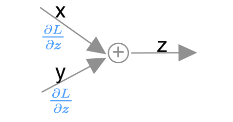
Sum
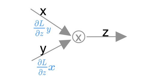
Multiplication
Forward AD
There are three ways to compute gradient. The simplest one is to apply common rules directly, for example,
$$ f(x) = x^2 \\ f'(x) = 2x $$
For composite functions, the gradient is computed step by step, for instance,
$$ f(x) = g(x) + h(x) \\ f'(x) = g'(x) + h'(x), \\ f(x) = g(x)\cdot h(x) \\f'(x) = h(x) g'(x) + h'(x) g(x) $$
However, it is difficult for complex functions to obtain such an equation. In this case, we solve it by applying numerical differentiation
$$ f'(x) = \text{lim}_{h\rarr0} \frac{f(x+h) - f(x)}{h} $$
Well, it seems perfect, but in practice, we do not know exactly what a function is composed of and the input variable could be dynamic. Ideally, we’d like to obtain the value of a function and the corresponding gradient simultaneously. This technique is known as automatic differentiation.
Forward mode AD is an intuive and simple way to accomplish this, which is similar to how computer works the equations out. For example, we have a funciton $z = xy + sin(x)$, and then computers will compute step by step as follows,
$$ x = ? \\ y = ?\\ a = xy \\ b = sin(x) \\ z = a + b $$
Let’s differentiate the each expression w.r.t some variable $t$
$$ \frac{dx}{dt} = ? \\ \frac{dy}{dt} = ? \\ \frac{\partial a}{\partial t} = x \frac{dy}{dt} + y \frac{dx}{dt} \\ \frac{\partial b}{\partial t} = cos(x) \frac{dx}{dt} \\ \frac{\partial z}{\partial t} = \frac{ \partial a }{\partial t} + \frac{ \partial b }{\partial t} $$
To get the derivative of $f$ w.r.t a specific variable, we simply set $t$ as the given varaible. For example, we set $t = x$ to compute $\frac{\partial z}{\partial x}$. Besides, we can see that the operation of excuating the function and computing the derivative can be done at the same time. Dual numbers is one way to achieve this concisely.
Dual number
Dual number is similar to complex number, which is defined as,
$$ a + b\epsilon $$
where $\epsilon^2 = 0$. Below are some basic rules of dual number
$$ (a + b\epsilon) + ( c + d\epsilon ) = a + c + (b + d)\epsilon \\ (a + b\epsilon)(c+d\epsilon) = ac + bc\epsilon + ad\epsilon $$
So… what is the use of dual number? We’ve known that Talyer expansion around a point $a$ is defined as
$$ f(x) = f(a) + f'(a) (x - a) + \sum_{n=2} \frac{f^n(a)}{n!} (x - a)^n $$
Let’s replace $x = a + b\epsilon$, then we have
$$ f(x) = f(a) + f'(a) b\epsilon + \epsilon^2 \sum_{n=2} \frac{f^n(a)}{n!} b^n\epsilon^{n-2} = f(a) + f'(a) b\epsilon $$
From this, we see that by calculating $x = a + b\epsilon$, we can obtain the value of the function $f(x)$ and the derivative at $x$ simultaneously. The implementation of forward mode AD by dual numbers is shown below,
class DualNumber:
    def __init__(self, value, dvalue):
        self.value = value
        self.dvalue = dvalue

    def __repr__(self):
        return repr(self.value) + ' + ' + repr(self.dvalue)  + "ε"

    def __str__(self):
        return str(self.value) + " + " + str(self.dvalue) + "ε"

    def __mul__(self, other):
        if isinstance(other, DualNumber):
            return DualNumber(self.value * other.value,
                self.dvalue * other.value + other.dvalue * self.value)

        return DualNumber(self.value * other, self.dvalue * other)

    def __add__(self, other):
        if isinstance(other, DualNumber):
            return DualNumber(self.value + other.value, self.dvalue + other.dvalue)

        return DualNumber(self.value + other, self.dvalue)


# test
x = 2
y = 5
a=DualNumber(x, 1)
b=DualNumber(y, 0) # w.r.t y
z = a * b + a  # df/da = b + 1
print(z) # it should be 6
# 12 + 6ε
Reverse AD(backprop)
Forward mode AD is intutive and simple, but we need to repeat $n$ times if there are $n$ variables. In other words, for each variable $x_i$, we need to set $t = x_i$ while keep others constant. If the process of computing deriative is complex and the number of parameters is huge (which is often the case in deep learning), it would take much time to obtain the whole derivatives. A solution is reverse mode AD, which enables us to obtain the derivatives of all variables in one go.
As previously mentioned, the chain rule is defined as
$$ \frac{\partial z}{\partial x_i} = \sum_{j}^n\frac{\partial z}{\partial y_j} \frac{\partial y_j}{\partial x_i} $$
We first consider each component $y_j$ that influence $z$, and then the change in each $y_i$ due of the change in an input variable $x_i$. Thus, $\frac{\partial y_j}{\partial x_i}$ could be zero for any $y_j$ that does not invovle $x_i$.
However, the chain rule can also be expressed as
$$ \frac{\partial z}{\partial x_i} = \sum_{j}^n \frac{\partial y_j}{\partial x_i} \frac{\partial z}{\partial y_j} $$
In this case, we first consider what output variables a given input variable $x_i$ can affect, and then how each output variable influence $z$. If $y_i$ has no contribution to $z$, $\frac{\partial z}{\partial y_j}$ is zero.
Therefore, suppose the yet-to-be-given output variable is $s$, we have
$$ \frac{\partial s}{\partial z} = ? \\ \frac{\partial s}{\partial b} = \frac{\partial z}{\partial b} \frac{\partial s}{\partial z} \\ \frac{\partial s}{\partial a} = \frac{\partial z}{\partial z} \frac{\partial s}{\partial z} \\ \frac{\partial s}{\partial y} = \frac{\partial a}{\partial y} \frac{\partial s}{\partial a} \\ \frac{\partial s}{\partial x} = \frac{\partial a}{\partial x} \frac{\partial s}{\partial a} + \frac{\partial b}{\partial x} \frac{\partial s}{\partial b} = (y + cos(x)) \frac{\partial s}{\partial z} $$
We can see the dependency between variables by drawing a tree, as shown in Figure 2. Besides, we also see that backprop follows breadth-depth first strategy. In other words, we compute gradients level by level.

When implementing reversel mode AD, we need to track the children nodes for each input variable and the derivative w.r.t each input input variable at this step, which are used to apply chain rule. Some example codes are shown below.
import math
class Var:
    def __init__(self, value):
        self.value = value
        self.children = []
        self.grad_value = None

    def grad(self):
      if self.grad_value is None:
          self.grad_value = sum(weight * var.grad() for weight, var in self.children)
      return self.grad_value

    def __repr__(self):
        return repr(self.value)

    def __str__(self):
        return str(self.value)

    def __mul__(self, other):
      z = Var(self.value * other.value)
      self.children.append((other.value, z)) # (derivative, output)
      other.children.append((self.value, z))
      return z

    def __add__(self, other):
        z = Var(self.value + other.value)
        self.children.append((1, z))
        other.children.append((1, z))
        return z

def sin(x):
  z = Var(math.sin(x.value))
  x.children.append((math.cos(x.value), z))
  return z


x = Var(2.0)
y = Var(3.0)
z = x*y + sin(x)
z.grad_value = 1.0 # see the gradient of z to 1
print(x.grad())