Deep Learning - RNN
When I first learned RNN, I found lots of articles about it. That’s good news, but most of them focus on the design of the architecture.The network itself is not difficult to understand, the real problem is why it works. What’s the intuition behind it? Why do we need “recurrence”? Unfortunately, few articles explain it clearly. Luckily, the book Deep Learning gives the answers.
RNN
Sequence Modeling
Recurrent neural networks (RNN) is another kind of neural networks, which are good at processing sequential data, such as stock prices, text, and audio. Machine translation and speech recognition are typical applications. So, what is special about sequential data? Why not still use MLP? Why do we bother designing another type of network to suit it?
Q1: the characteristics of sequential data
Sequential data consists of a series of data points across time, which have a dependency on each other. In CNN, we feed a single image into the network each time, but the order of these images doesn’t matter. Each image is an independent individual. However, when we process text, the order of words matters. For example, “I like running” is a correct sentence while “Running like I” is wrong. More importantly, there are dependencies between words. We understand the meaning of a piece of text or audio based on the understanding of the previous words.
Q2: Why not MLP?
Remember that there are two main reasons why we use CNN rather than MLP
- MLP cannot capture spatial information
- Flattening will cause the loss of spatial information of image pixels, especially there are multiple channels (depth). For example, the colour of a pixel can be estimated by considering the nearest neighbouring pixel’s value
- Repeated pattern is hard to detect
- The object to be detected (e.g. Cats) can appear anywhere in the image. Actually, we do not care about locations but the pattern.
Well, the reasons why MLP is not suitable for sequential data are similar.
- Spatial information in sequential data means the order of data and dependencies among data.
- Each word is considered as an input feature when using MLP, but the representation of each word does not contain dependencies between words.
- A sentence can be written in different ways using the same words.
- For example, “Today, I am going to watch a movie.” is the same as “I am going to watch a movie today.” When we feed each word into MLP, “Today” will be assigned with different weights.
- Sentence length is variable.
Q3: What kind of networks is suitable for sequential data?
From the above analysis, we conclude that a network that is capable of modeling sequential data should be able to
- handle with variable sequence length
- retain the order of data and dependencies between data
- detect repeated patterns
Architecture
So, how RNN works? Figure 1 shows that RNN is somehow a kind of state machine, which only accepts two inputs:
- the previous system state $h_{t-1}$
- the current input $x_t$

Specifically, RNN is defined as
$$ h_t = \sigma (W_x x_t + W_h h_{t-1} + b_h) \\ o_t = W_y h_t + b_y \\ \hat y_t = \sigma(o_t) $$ First, unlike the Feed Forward Networks that requires fixed length of the inputs, RNN can accormadate variable sequence length by looping. Second, the input data are fed into the network sequentially to maintain the order. At each time $t$, the system will reach a new state $h_t$ by receiving the previous state $h_{t-1}$ and the current input $x_t$. And the new state will be fed into the network recursively. In other words, at each time $t$, the system has already known what happend before through $h_{t-1}$. Finally, the weights of RNN are shared ( $W_t, W_h, W_y, b_h, b_y$ ) each time step to capture the repeated pattern.
BPTT
Traning a RNN is nothing special. First, let’s define the loss function. For a sequence whose length is $T$, the loss is computed as
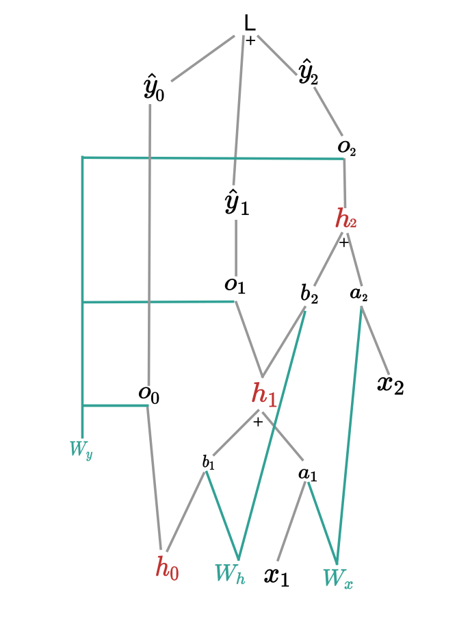
$$ L = \sum_{t=1}^T L_t (\hat y_t, y_t) = \sum_{t=1}^T -y_t \text{log}\hat y_t = \sum_{t=1}^T -y_t \text{log} \sigma(o_t) $$ where $\sigma$ is the softmax function. The computation graph is shown below.
$W_y$
First, we compute the gradient of $L$ w.r.t $W_y$. From Figure 2, we can see that $W_y$ has three parents $o_0, o_1, o_2$. We can generalize it to $T$ time steps $$ \frac {\partial L}{\partial W_y} = \sum_{t=1}^T \frac {\partial o_t}{\partial W_y} \frac {\partial L}{\partial o_t} = \sum_{t=1}^T \frac {\partial o_t}{\partial W_y} \frac {\partial \hat y_t}{\partial o_t} \frac {\partial L}{\partial \hat y_t} $$
Now the question is — what’s the derivative of $L$ w.r.t $o_t$?
$$ \frac {\partial L}{\partial o_t} = -y_t \frac{1}{\sigma(o_t)} \frac{\partial \sigma(o_t)}{\partial o_t} - \sum_{i \neq t} ^N y_i \frac{1}{\sigma(o_i)} \frac{\partial \sigma(o_i)}{\partial o_t} $$
Generally, $\sigma$ is the softmax function, so the derivative of $\sigma$ w.r.t $o_i$ is given as
$$ \frac{\partial \frac{e^{o_t}}{\sum_{k=1}^K e^{o_k}}}{\partial o_i} = \frac{ \frac{\partial e^{o_t}}{\partial o_i} \sum_{k=1}^K e^{o_k} - e^{o_i} e^{o_t} }{ [\sum_{k=1}^K e^{o_k} ]^2} $$
Here, we use the derivative of $f(x) = \frac{g(x)}{h(x)}$ directly.
$$ f'(x) = \frac{g'(x)h(x) - h'(x)g(x)}{h^2(x)} $$
For $i = t$, we have
$$ \frac{\partial \sigma(o_t)}{\partial o_t} = \sigma(o_t) (1 - \sigma(o_t)) $$ For $i \ne t$, we have
$$ \frac{\partial \sigma(o_i)}{\partial o_t} = - \sigma(o_i) \sigma(o_t) $$ Thus,
$$ \frac {\partial L}{\partial o_t} = -y_t \frac{1}{\sigma(o_t)} \sigma(o_t) (1 - \sigma(o_t)) + \sum_{i \neq t} ^N y_i \frac{1}{\sigma(o_i)} \sigma(o_i) \sigma(o_t) = -y_t (1 - \sigma(o_t)) + \sum_{i \neq t} ^N y_i \sigma(o_t) \\ = -y_t + y_t \sigma(o_t) + \sum_{i \neq t} ^N y_i \sigma(o_t) = \sigma(o_t) - y_t $$
Finally, we have $$ \frac {\partial L}{\partial W_y} = \sum_{t=1}^T \frac {\partial o_t}{\partial W_y} \frac {\partial L}{\partial o_t} = \sum_{t=1}^T (\hat y_t - y_t) \otimes h_t $$
where $\otimes$ is the outer product of vectors.
$W_h$
Similarly, the gradient of $L_2$ w.r.t $W_h$ is the sum of gradients of all nodes that are the parents of $W_h$.
$$ \frac {\partial L_2}{\partial W_h} = \frac {\partial h_0}{\partial W_h} \frac {\partial L_2}{\partial h_0}+ \frac {\partial h_1}{\partial W_h} \frac {\partial L_2}{\partial h_1} + \frac {\partial h_2}{\partial W_h} \frac {\partial L_2}{\partial h_2} \\ \ \\ = \frac {\partial h_0}{\partial W_h} \frac {\partial h_1}{\partial h_0} \frac {\partial h_2}{\partial h_1}\frac {\partial L_2}{\partial h_2} + \frac {\partial h_1}{\partial W_h} \frac {\partial h_2}{\partial h_1} \frac {\partial L_2}{\partial h_2} + \frac {\partial h_2}{\partial W_h} \frac {\partial L_2}{\partial h_2} \\ \ \\ = \sum_{i=0}^2 \frac {\partial h_i}{\partial W_h} (\prod_{j=i}^2 \frac {\partial h_{j+1}}{\partial h_j} ) \frac {\partial L_2}{\partial h_2} \\ \ \\ = \sum_{i=0}^2 \frac {\partial h_i}{\partial W_h} (\prod_{j=i}^2 \frac {\partial h_{j+1}}{\partial h_j} ) \frac {\partial \hat y_2}{\partial h_2} \frac {\partial L_2}{\partial \hat y_2} $$
So, the gradient of $L$ w.r.t $W_h$ is
$$ \frac {\partial L}{\partial W_h} = \sum_{t=0}^T \sum_{i=0}^t \frac {\partial h_i}{\partial W_h} (\prod_{j=i}^t \frac {\partial h_{j+1}}{\partial h_j} ) \frac {\partial \hat y_t}{\partial h_t} \frac {\partial L_t}{\partial \hat y_t} $$
$W_x$
Similarly, the gradient of $L$ w.r.t $W_x$ is defined as follows,
$$ \frac {\partial L}{\partial W_x} = \sum_{t=0}^T \sum_{i=0}^t \frac {\partial h_i}{\partial W_x} (\prod_{j=i}^t \frac {\partial h_{j+1}}{\partial h_j} ) \frac {\partial \hat y_t}{\partial h_t} \frac {\partial L_t}{\partial \hat y_t} $$
Truncated BPTT
Vanishing/Exploding Gradient
Problem
The main problem of RNN is the well-known vanishing/exploding gradient. Why? From the above equations, we can see that it could be due to the repeated multiplication of $\frac {\partial h_{j+1}}{\partial h_j}$.
Remember that $h_{j+1}$ is derived from
$$ h_{j+1} = \text{tanh} (W_h h_j + W_x x_{j+1} + b_h) $$ Thus, the derivative is
$$ \frac {\partial h_{j+1}}{\partial h_j} = \text{diag} [\text{tanh}'(o_j)] W_h $$
So, the gradient is determined by the weights and the derivatives of the activation functions. (PS: the result is a Jacobian matrix because we are taking the derivative of a vector function w.r.t a vector.)
First, the activation function is usually tanh or sigomid funtion, and they have the following properties:
- the derivatives are always less than 1
- the derivatives tend to be saturated and close to zero when the input are far away from zero.
Thus, with small values in the matrix and multiple multiplications, the gradient will shrink quickly.
Second, if $W_h$ overpowers $\text{tanh}'(o_j)$, the gradient value can be inferred by the eigenvalues of $W_h$, as the below equation shows,
$$ \prod_{j=i}^t \frac {\partial h_{j+1}}{\partial h_j} = Q \Lambda^{t-i} Q^{-1} $$
- If the largest eigenvalue of $W_h$ is greater than 1, the gradient will grow quickly and go to infinity
- On the contrary, if it is less than 1, the gradient will shrink exponentially
Identify vanishing/exploding
So, there are some signals that might indicate that we are suffering from vanishing or exploding
vanishing
- the parameters of the deepest layers changes greatly but the parameters of the front layers change little
- the model learns slowly
exploding
- the parameters changes exponentially
- the parameters might be NaN
Solution
Gradient Clipping
There is a specific solution to mitigate the exploding gradient —— gradient clipping. Since the gradient is too huge, it’s likely to move out of the parameter plane. An intuitive way is to control the size of the gradient (threshold), which is denoted by $\eta$. The intuition is to take a step in the same directions, but a smaller step.
$$ \text{if } ||g|| \ge \eta: g = \eta \frac{g}{||g||} $$
Non-saturating Activation Function
Instead of using sigmoid and tanh functions that prone to be saturated, we use non-saturating functions, such as ReLu.
Weight Initialization
Batch Normalization
The purpose of normalization is to transform data into a fixed range by translation and scale. It is a common technique used in data preprocessing. Min-max and z-score are two common normalization methods. Batch normalization means normalization performed on a batch of data rather than the whole data as we train data by group in NN. Below is the algorithm of batch normalization,
$$ \mu = \frac{1}{|B|} \sum x_i \\ \sigma^2 = \frac{1}{|B|}\sum(x_i - \mu)^2 \\ x_i' = \frac{x_i - \mu}{\sqrt { \sigma^2 + \epsilon}} \\ y_i = r x_i' + \beta $$
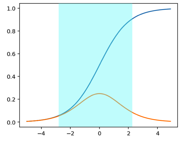
Figure 3 shows what batch normalization does. Before normalization, $x$ could be anywhere in the input space. After normalization, we restrict the input space to a small range (the shadow area), preventing $x$ from reaching the edges of the sigmoid function. In doing so, the gradient of the sigmoid function is unlikely to be small value.
Pros
- avoid vanishing gradient
Cons
- depends on the batch size, small batch size may cause unstable results
- not suitable for dynamic networks, e.g. RNN (different time steps)
Re-design Networks
Some effective new networks are residual networks or gated RNNs.
Gated RNN
Intuition
The introduce of gate in gated RNNs can be considered in this way: the input data at each time step are not of equal importance. For example, in a sentence, the first word might be more important than the second word, so we’d better to keep the previous system stable and not change too much at the second time step. Thus, we need some controls on the current system state and the current input data, determining how much they could affect on the system.
Strictly speaking, the purpose of the gates is to ensure the integrity of information, as Written Memories: Understanding, Deriving and Extending the LSTM said. In RNN, $h_t$ is paricipated in the creation of new information at each time step. However, the new state will be ultimately fed into the non-linear function, such as tanh, causing the problem of information morphing. Therefore, it is difficult to decode the past information even if it is included in the current system state due to the distortion of information.
How to solve it? We explicitly add and subtract information from the system. We also need a read interface to avoid information overload. This is because the system contains so much information that not all of them are useful to the current time step. Moreover, we should read something first before writing, because we know nothing about the current system (we shall know something before writting). Otherwise, we run the risk of overwriting the system without having the old information (break the incremental change).
At the very beginning, we can read from the initial state. After that, we read the previous state ($s_{t-1}$), then decide what new information to write based on it. The new information is known as the candidate state, denoted by $\widetilde s_t$. We selectively forget some useless information (sbstraction), and update the system using the candidate state (addition). In doing so, we can ensure that the change in the system state is incremental, $$ s_t = s_{t-1} + \Delta s_t $$
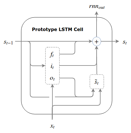
Figure 4 depicts the internal structure of the initial LSTM. Below are the complete equations from Written Memories
$$ f_t = \sigma (W^fs_{t-1}+ U^fx_t + b^f) \\ i_t = \sigma (W^i s_{t-1} + U^ix_t + b^i) \\ o_t = \sigma (W^o s_{t-1} + U^o x_t + b^o) \\ \ \\ \widetilde s_t = \phi (W(o_t \odot s_{t-1}) + Ux_t + b) \\ s_t = f_t \odot s_{t-1} + i_t \odot \widetilde s_t $$
LSTM
LSTM, short for long short-term memory, is designed to retain long-time dependencies. The main differences with vanilla RNNs are the cell state and the design of three gates, as shown in Figure 5.
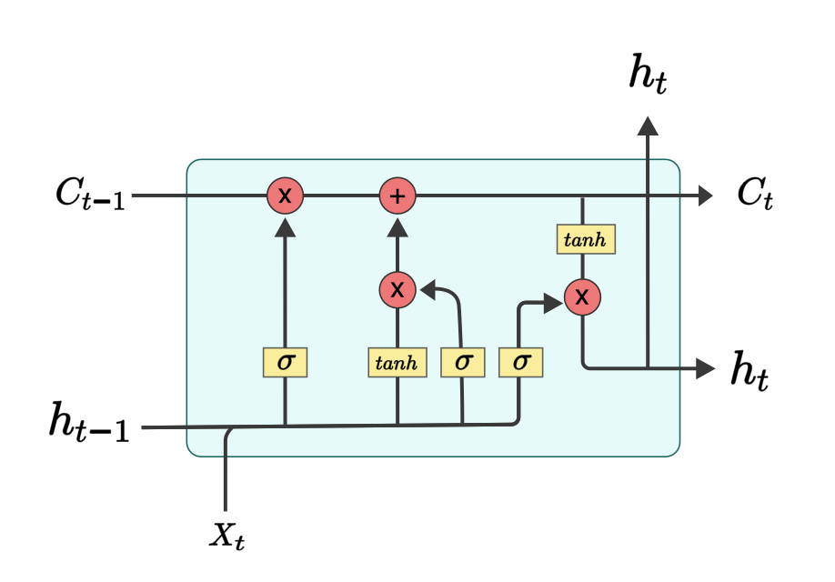
- There are three gates in LSTM, namely, forget gate, input gate and output gate. The value of gates is between 0 and 1, which is often achieved using the sigmoid function. 0 means nothing will flow through the gate, while 1 indicates all information will pass.
- $$f_t = \sigma (W_x^fx_t + W_h^fh_{t-1} + b^f)$$
- $$i_t = \sigma (W_x^ix_t + W_h^ih_{t-1} + b^i)$$
- $$o_t = \sigma (W_x^ox_t + W_h^oh_{t-1} + b^o)$$
- The new information at the current step is the same as the vanilla RNN
- $$g_t = \text{tanh} (W_x^gx_t + W_h^gh_{t-1} + b^g)$$
- The cell state, denoted by $C_t$, is the horizontal line across LSTM. It contains the whole information of the system and is visible to LSTM only. As mentioned above, we can control the extent to which we want to forget the previous information and how much the new information to be added. For example, if $f$ is close to 1 and $i$ is close to 0, the previous information retains, which means the inputs at the current step might not be so important (the first word might be more important than the second word)
- $$C_t = f_t \odot C_{t-1} + i_t \odot g_t$$
- The current hidden state (used for making decision) is derived from the cell state and the current inputs.
$$ h_t = o_t \odot \text{tanh} (C_t) $$
Unlike the prototype LSTM, the real LSTM in practice has several differences.
- the state to be used for writting has already been ready, that is the hidden state $h_{t-1}$ ( $h_{t-1} = o_{t-1} \odot s_{t-1}$)
- we can immediately obtain the candidate write $g_t$, and then update the main state $c_t$
- finally, we obtain the next hidden state from $c_t$ using $o_t$
So why does LSTM mitigate the problem of vanishing gradient? The reason why gradient vanishes is the recursive multiplication of weight and derivative of the activation functions, as explained above. However, in LSTM, gradient is calculated by addition instead of multiplication, as shown below.
$$ \frac{\partial C_t}{\partial C_{t-1}} = \frac{\partial f_t \odot C_{t-1}}{\partial C_{t-1}} + \frac{\partial i_t \odot g_t}{\partial C_{t-1}} \\ = \frac{\partial f_t }{\partial C_{t-1}} \odot C_{t-1} + \frac{\partial C_{t-1} }{\partial C_{t-1}} \odot f_t + \frac{\partial i_t \odot g_t}{\partial C_{t-1}} \\ = f_t + C_{t-1} \odot \frac{\partial f_t}{\partial h_{t-1}}\frac{\partial h_{t-1}}{\partial C_{t-1}} + g_t \odot \frac{\partial i_t}{\partial h_{t-1}}\frac{\partial h_{t-1}}{\partial C_{t-1}} + i_t \odot \frac{\partial g_t}{\partial h_{t-1}}\frac{\partial h_{t-1}}{\partial C_{t-1}} \\ = f_t + C_{t-1} \odot \sigma' W_h^f o_{t-1} \odot \text{tanh}'(C_{t-1}) + g_t \odot \sigma' W_h^i o_{t-1} \odot \text{tanh}'(C_{t-1}) + i_t \odot \sigma' W_h^g o_{t-1} \odot \text{tanh}'(C_{t-1}) $$
Let’s compare it with the vanilla RNN
$$ \frac {\partial h_{j+1}}{\partial h_j} = \text{diag} [\text{tanh}'(o_j)] W_h $$
From the above equations, we can see that the gradient in LSTM is more flexible than RNN in two aspects
- $f_t, i_t, g_t$ are learned from the current time step
- gradient can vary at each time step in LSTM (at step 1, it could be greater 1; at step 2, it might be less than 1), while it’s either less than 1 or greater than 1 in RNN
In this way, it is possible for LSTM to retain gradient for a long time.
GRU
There are many variants of LSTM, and one of them is GRU, as Figure 6 shows.
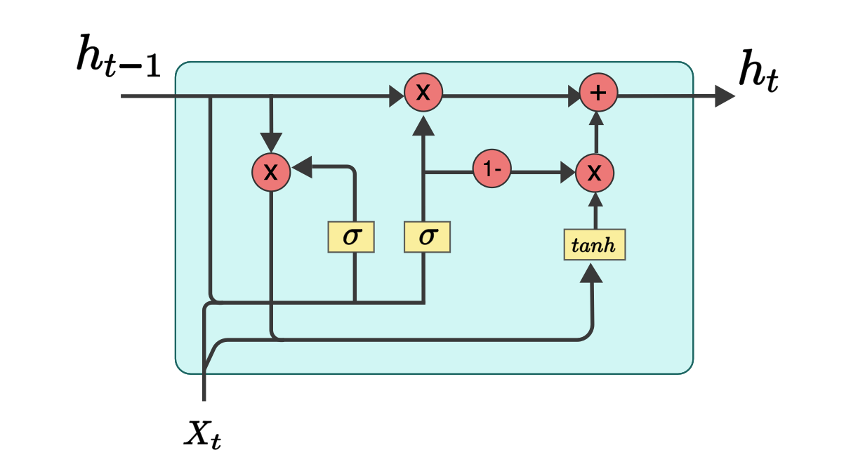
From Figure 6, we see that there are 2 gates and only one state in GRU.
- the reset gate $r_t$, which is also the read gate in the prototype LSTM
- the update gate $z_t$, which is the concise version of forget ($z_t$) and update ($1-z_t$) gates in the prototype LSTM
Thus, the equations in GRU can be derived as follows,
$$ r_t = \sigma (W^rh_{t-1}+ U^rx_t + b^r) \\ z_t = \sigma (W^z h_{t-1} + U^zx_t + b^z) \\ \ \\ \widetilde h_t = \phi (W(r_t \odot h_{t-1}) + Ux_t + b) \\ h_t = z_t \odot h_{t-1} + (1 - z_t) \odot \widetilde h_t $$
BiRNN
References
- Exploding and Vanishing Gradients
- Backpropagation Through Time for Recurrent Neural Network
- Fancy RNN
- Written Memories: Understanding, Deriving and Extending the LSTM
- The Vanishing Gradient Problem
- Why LSTM Solves the Gradient Vanishing Problem of RNN
- And of course, LSTM — Part II
- Deriving the backpropagation equations for a LSTM
- Deriving LSTM Gradient for Backpropagation