Decision Tree
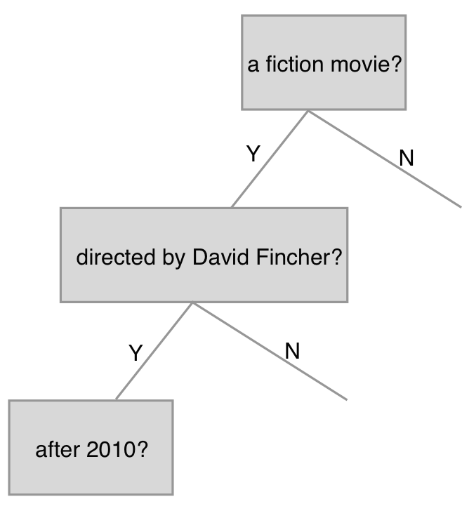
The way decision tree works is similar to the way we make decisions in real life. For example,when you are going to watch a movie, you might have some questions on your head, such as ‘Is it a fiction movie? Is it directed by David Fincher?’

From Figure 1, we can see that a decision tree builds a binary tree to partion the data. Each node is a decision rule based on a feature and the tree can grow endlessly. Two questions then arise:
- How is the decision rule made?
- How deep is the decision tree?
Decision Rule
Since there are so many features and each feature can have different values, we have to loop over all of them and find the best split. Well, how to measure the performance of a split? There are 3 measures widely used — Gini Impurity, Entropy, and Information Gain.
Gini Index
Gini Index, also known as Gini Impurity, measures how often a randomly selected element from the set is classified incorrectly.
$$ Q_m^g(L) = \sum_{c \in C } p_c(L) (1 - p_c(L)) = 1 - \sum_{c \in C } p_c(L)^2 $$
where $L$ is short for the children node and $p_c(L)$ is the faction of class $c$ in the leaf node $L$,
$$ p_c(L) = \frac{1}{|L|} \sum_{x, y \in L} [y == c] $$
where $[y == c] = 1$ if $y$ belongs to class $c$ and 0 otherwise.

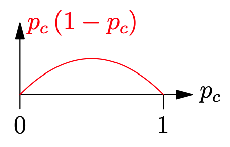
Figure 2 shows that the value of Gini Index is the lowest at the start and end of the x-axis and maximum at the middle of the x-axis. In other words,
- If the leaf node only has one class, then this node is a pure node and the gini impurity of this leaf node is 0.
- On the other hand, if all elements in this leaf node belong to an individual class, then the Gini Index of this node has the maximum value of $ 1 - 1/len(L) $.
Entropy
Entropy is a concept of Information Theory. Before introducing the entropy, we should have a little understanding of information.
Information is related to the surprise in some way. For example, if I told you that you will go to work tomorrow. Well, that’s not surprising because you work every day. However, if I told you that tomorrow is the end of the world, you are likely to be shocked because it is an breaking news.
We can measure this surprise by the following equation
$$ I(x) = -log(p(x)) $$
If an event is unlikely to happen, then $p(x)$ is close to 0 and $I(x)$ tends to be infinity, which means it conveys much information since impossible things happened and it must have a significant implication behind it.
Then what’s the entropy? The previous equation calculate the information contained in one outcome. However, it’s quite often to have many outcomes for a random variable $X$. Therefore, the expected information over all outcomes is defined as the entropy.
$$ H(X) = E_{x \in X}[-log(p(x)] $$
In this case, the classes in the leaf node is the random variable $X$ and the probability of each outcome is the fraction of each class, which is expressed as
$$ Q_m^e(L) = \sum_{c \in C}- p_c(L) log(p_c(L)) $$
In a word, entropy measures the randomness of a set. Lower entropy means a purer set while higher entropy means there are more other classes that is not the class $c$ in a set.
Information Gain
Information Gain is simply the difference between the impurity of the parent node $A$ before splitting and the sum of impurity of all children nodes after splitting. It measures how much the impurity of a set $A$ were reduced after splitting. The larger the information gain is, the better the split is.
$$ IG(A) = H(A) - \sum_{L \in children \ nodes} p(L) H(L) $$
In summary, when a decisiton tree makes a split on a feature, it tries to achieve,
- a lower impurity
- a lower entropy
- a higher information gain
CART Algorithm
CART is short for classification and regression tree algorithm, which is used to train Decisioin Trees. CART tries to find the best split that produces purest subsets by calculating the weighted Gini Impurity on each split made by each feature $k$ from the parent node’s training sample and corresponding threshold $t_k$.
Specifically, it tries to minimize the following loss function for a classification task,
$$ L(k, t_k) = \frac{|C_m^L|}{|N_m|}Q_m(C_m^L) + \frac{|C_m^R|}{|N_m|} Q_m(C_m^R) $$
where $C_m^L$ and $C_m^R$ are children nodes splitted on node $N_m$.
For a regression task, it minimizes the sum of squred error
$$ L(k, t_k) = \frac{|C_m^L|}{|N_m|}SSE(C_m^L) + \frac{|C_m^R|}{|N_m|} SSE(C_m^R) $$
where $SSE(subset)$ is defined as
$$ SSE(subset) = \sum_{n \in subset} (y_n - \overline y)^2 $$
$$ \overline y = \frac{1}{|subset|} \sum_{n \in subset} y_n $$
Prunning
Now let’s address the second problem, i.e. when to stop growing the tree. You can either stop growing the tree when you build the tree or trim the tree after building, which are known as pre-pruning and post-pruning respectively.
Pre-pruning
Scikit-learn provides several hyperparameters to do a pre-pruning:
- the maximum depth
- the minimum number of the samples a node must have to split
- the minimum number of the samples in a leaf node
- the maximum number of leaf nodes
All of these parameters can be tuned with cross-validation.
TODO
Post-pruning
Though pre-pruning is straightforward, it is a bit short-sighted since it doesn’t build a full tree and there might be some splits works better later on. Therefore, it would be better to have a large and full-size tree and then we trim some less important branches to avoid overfitting. Cost complexity pruning, also known as weakest link pruning, is one way to achieve this.
Pros and Cons
Advantages:
- Decision trees are simple and intutive to interpret, and we can easily visualize the process of decision making.
- They can be used for both classification and regression.
- There is no need to normalize or scale data.
- They can help to understand what features are most important.
Disadvantages:
- They can be easy to overfit.
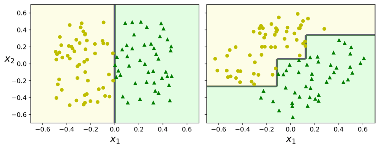
- They are sensitive to variations of training data. If you rotate the same data, you will get a completely different tree because all splits are perpendicular to an axis.

References
[1] A. Géron, Hands-on machine learning with Scikit-Learn and TensorFlow. Sebastopol (CA): O’Reilly Media, 2019.
[2] arunmohan, “Pruning decision trees,” Kaggle.com, 02-Sep-2020. [Online]. Available: https://www.kaggle.com/arunmohan003/pruning-decision-trees. [Accessed: 22-Apr-2021].
[3] “How to choose α in cost-complexity pruning?,” Stackexchange.com. [Online]. Available: https://stats.stackexchange.com/questions/193538/how-to-choose-alpha-in-cost-complexity-pruning. [Accessed: 22-Apr-2021].
[4] “Cost-complexity pruning - ML wiki,” Mlwiki.org. [Online]. Available: http://mlwiki.org/index.php/Cost-Complexity_Pruning. [Accessed: 22-Apr-2021].