Descriptive Statistics
Statistics is one of the most important skills for data scientists. There are two main branches:
- descriptive statistics tells us the statistics about data like mean, mode and standard deviation, which you’ve learned in high school.
- inferential statistics, on the other hand, uses a random dataset sampled from the population to make inferences about the population.
In this post, we focus on descriptive statistics and other basic concepts in statistics.
Central tendency
Central tendency measures the centre of the data. Mean, mode, and median are three mainly used metrics.
Mean
Mean is the average of data and calculated by summing up all data values and then dividing them by the number of data. For instance, say we have data 1,2,3,4,5,6, the mean is 3.5.
$$ \overline x = \frac{\sum_i^nx_i}{n} $$
# vanilla python
def mean(x):
	return sum(x)/len(x)
Median
Though mean is widely used, it’s sensitive to outliers. Suppose you have a set of data 1,2,3,4,5,6,100, after some calculations, you find that the mean is 17.28. However, it seems not convincing as most of the data values are less than 10 except for one extreme value 100.
To get the median, firstly we need to sort the data in ascending order and then find the middle number that separates the data into two groups of the same size. In this example, the median is 4.
def median(x):
  mid_p = len(x) // 2
  if len(x) % 2 == 0: # even
    return (x[mid_p] + x[mid_p-1])/2
  else: # odd
    return x[mid_p]
Mode
Mode is the most frequent value. There could be one, two or more data values with the same frequency, and that frequency is the largest. For instance,
from collections import Counter
a = [1, 2, 4, 5, 6, 6, 7, 6, 4, 4, 3, 3, 3, 2, 2,2, 10, 2, 3, 3]
Counter(a).most_common()
# [(2, 5), (3, 5), (4, 3), (6, 3), (1, 1), (5, 1), (7, 1), (10, 1)]
Dispersion
Dispersion measures how spread out a given dataset is.
Range
Range is the distance between the maximum value and the minimum value. Again, the range is sensitive to outliers.
$$ r=max - min $$
Quantile
Quantiles are used to divide data into several equal-sized groups. The most widely used cut points are 0, 25, 50, 75, 100, denoted by min, Q1, Q2, Q3, max, respectively. IQR (interquartile range) measures where the central 50% of the data is.
$$ \text{IQR} = Q3 - Q1 $$
IQR can be used to detect outliers. Data that is greater than the upper boundary or less than the lower boundary can be considered as outliers.
$$ \text{upper boundary }= Q3 + 1.5*IQR $$
$$ \text{lower boundary} = Q1 - 1.5*IQR $$
Variance
The deviation is the distance between a given data point and the mean. Since there are many data points, the variance calculates the average deviation from the mean. But when you do this, you will always get a zero due to the definition of the mean.
$$ \frac{1}{n}\sum_i^n d_i = \frac{1}{n}\sum_i^n (x_i - \overline x) = \frac{1}{n}\sum_i^nx_i - n\overline x = \frac{1}{n} (n\overline x - n\overline x) = 0 $$
Let’s try to ignore the sign and use the absolute value of the deviation.
$$ \frac{1}{n-1} \sum_i^n d_i = \frac{1}{n-1} \sum_i^n |x - \overline x| $$
Though it works, the most widely used method is to calculate the square of the deviation.
$$ s^2 = \frac{1}{n-1} \sum_i^n (x_i - \overline x)^2 $$
However, the squared value is a bit hard to interpret. For instance, below are 15 records of fish size measured in kilogram, and the variance is 30.97. It means that if we randomly catch a fish, its weight would be 30.97 squared kilograms far away from the average weight. Emm…, a squared kilogram is an odd unit.
2.1, 2.4, 2.4, 2.4, 2.4, 2.6, 2.9, 3.2, 3.2, 3.9, 4.5, 6.3, 8.2, 12.8, 23.5
Standard Deviation
It’s simple to solve this problem by taking the square root of the variance, which is the standard deviation. The standard deviation in the previous example is 5.56kg, which makes more sense.
$$ s = \sqrt{\frac{\sum (x - \overline x)^2}{n-1}} $$
Distribution
Skewness
Skewness measures the symmetry of a distribution. It’s quite common to have non-symmetric distributions shown in Figure 1.

A left-/negative-skewed distribution
- a long left tail
- mean < median
A right-/positive-skewed distribution
- a long right tail
- mean > median
A skewed distribution implies that some special values are much larger/smaller than the common values. Let’s see an example.
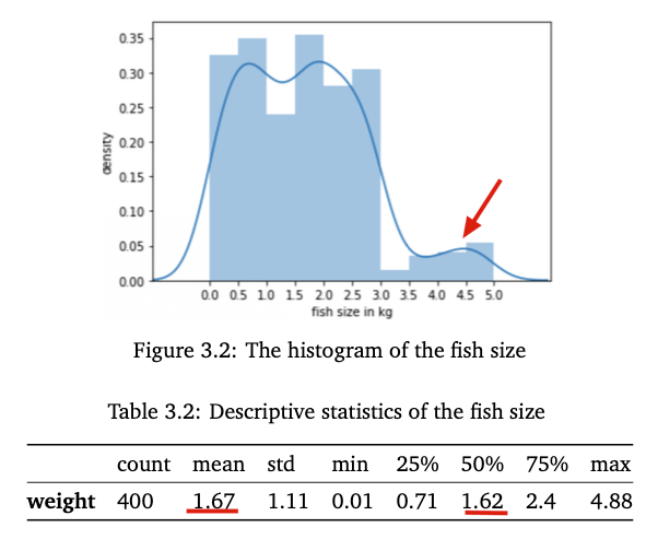
Figure 3.2 shows the histogram of the fish sizes gathered from a fisherman. We can see that this distribution is right-skewed. The majority of fish sizes are between 0 and 3kg, but a few fishes weigh over 3.5kg. It also can be seen that the average weight(1.67kg) is a bit higher than the median(1.62kg) shown in Table 3.2.
Correlation
So far we have introduced different methods of characterizing the distribution of a single variable. But what about two or more variables? You might want to find the relationships between them. An intuitive way is to visualise data using a scatterplot. For example, you might find that car prices tend to increase as car ages decrease.
Statistically, we can measure both the direction and the strength of this tendency using correlation coefficients. And Pearson correlation coefficients is widely used to measure the strength of a linear relationship. It can be calculated as follows,
$$ r = \frac{Cov(X, Y)}{\sqrt{V(X)}\sqrt{V(Y)} } $$
where $Cov(X, Y)$ is the covariance between $X$ and $Y$, and $V(X), V(Y)$ are the standard deviation of $X, Y$ respectively. The value of $r$ ranges between -1 and 1.
- a negative value represents a negative relationship
- a positive value represents a positive relationship
- $0$ means there is no relationship between $X$ and $Y$
But to what extent is the value of $r$ large means a strong relationship? Below are some values that could give you an insight into how strong your correlation $r$ is.
- 0 - 0.3: weak relationship
- 0.3 - 0.6: moderate relationship
- 0.6 - 0.9: strong relationship
- 0.9 - 1.0: very relationship
Data Types
Now let’s look at some characteristics of data. Roughly, we classify data into two categories:
- numerical/quantitative data
- categorical/qualitative data
Categorical data refers to data that cannot be measured, for example, the color of car or the quality of service. There are two subcategories, namely nominal data and ordinal data. The difference between them is that ordinal data can have order, such as 0=bad, 1=good, 2=better, 3=excellent.
Numerical data refers to data that can be measured. There are also two subcategories, namely discrete and continuous. Discrete data describes values that cannot be divided into smaller individual parts, e.g. the number of people. You cannot say, ‘There are 1.5 people’. However, we can say, ‘He is 1.87 meters tall’. So height is a continuous variable.
Measurement Scales
At a lower level, we can also classify data from the perspective of measurement scales, which capture the characteristics of data used to determine the types of variables. There are four main levels of measurement scales:
- nominal
- ordinal
- interval
- ratio
Each of them satisfies one or more of the following properties of measurement.
- Identity
- each value have a unique meaning
- $=, \cancel{=}$
- nominal scale, e.g. car color
- Maginitue
- values have an ordered relationship to one another
- $\lt, \le, \gt, \ge$
- ordinal scale, e.g. service quality
- Equal interval
- the different between data points A and B will be equal to the different between data points C and D
- $+, -$
- interval scale, e.g. time
- A minimum value of zero
- the scale has a true zero point, below which no value exists
- ratio scale, e.g. height
References
[1] B. al., “Introduction to Statistics | Simple Book Production”, Courses.lumenlearning.com, 2021. [Online]. Available: https://courses.lumenlearning.com/introstats1. [Accessed: 14- Apr- 2021].
[2]“Measurement Scales”, Stattrek.com, 2021. [Online]. Available: https://stattrek.com/statistics/measurement-scales.aspx?tutorial=reg. [Accessed: 11- May- 2021].