Ensemble Methods
Ensemble means a group of people or a collection of things.Thus, ensemble methods means rather than using a single model, we will use a group of different models to gain a better prediction. In fact, ensemble methods often outperform other models in Kaggle competitions. In this post, we will talk about the most popular ensemble methods , including voting, bagging, and boosting.
Overview
In real life, we often take advices from others. For example, suppose you want to know whether a movie is worthwhile to watch, you may ask your friends who’ve watched to give the movie a score(out of 5), say 3, 3, 2, 2, 2, 4. Since 5 people gave a score that is lower than 4, you may think about choosing another movie, let’s say Avatar. Then you ask your friends again and have some scores like this 5, 5, 5, 5, 5. Wow! All of your friends think that Avatar is an amazing movie that should certainly not be missed. You agree with their opinons and decide to watch Avatar finally. From this example, we can see that gathering plenty of opinions from different people are likely to make an informed decision.
Here, I highlight the words different people. It makes little sense if we only asks for people who have the same interests. Therefore, the more diverse the people are, the more sensible our decisions are. Basically, the idea behind it is the wisdom of collaborating.
Voting
The method used to decide whether to watch a movie or not in this example is known as voting. For classification, there are 2 types of voting named hard voting and soft voting.
- Hard voting returns the most popular class shown in Figure 1.
- Soft voting averages the probability of each class and then return the class that has the maximum probability.
Hard Voting
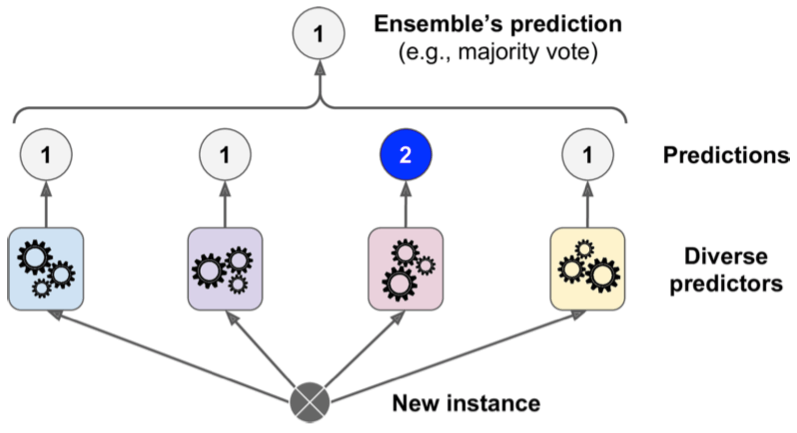
Figure 1 can also be illustrated in a mathematical way,
$$ y' = mode(C_1(x), C_2(x), …, C_n(x)) $$
For example, {0, 1, 0, 1, 1} are the class labels predicted by our 5 different classifiers for a data point $x$. By hard voting, the final class label is class 1 .
C1 -> 0
C2 -> 1
C3 -> 0
C4 -> 1
C5 -> 1
Weighted Hard Voting
Hard voting works nice, but in some cases, some people might be more professional than others. Hence, their opinions are much more significant. How to distinguish professionals and common people?
We assign weights to them. Specifically, we assign higher weights to professionals while common people have lower weights. Then we calculate weighted sum of occurrence of each class label and find the class label that has the maximum value.
$$ y' = \operatorname*{argmax}_i w_j\sum_j [C_j == i] $$
where $[C_j == i] = 1$ if classifier $j$ predicts class label i and 0 otherwise.
For example, if we assign the following weights to the previous 5 classifiers, then we will have 0.7 for class 0 and0.5 for class 1. Thus, class 0 wins because 0.7 is greater than 0.5.
0.4, C1 -> 0
0.1, C2 -> 1
0.3, C3 -> 0
0.2, C4 -> 1
0.2, C5 -> 1
Soft Voting
Instead of predicting the class label directly, some classifiers like logistic regression can predict the probability of each class label that $x$ belongs to. Then we simply average these probabilities for each class label. Certainly, you can assign weights to classifiers.
$$ y' = \operatorname*{argmax}_i \frac{1}{n} \sum_j^n w_j p_{ij} $$
where $p_{ij}$ is the probability of class label $i$ that $x$ belongs to when using classifier $C_j$.
Average for Regression
We simply average the predictions of different machines for a regression task.
$$ y' = \frac{1}{n} \sum_j^n w_j C_j $$
Bagging
In order to make our models different from each other, we use various algorithms to train the same data, as discussed above. Another way to have a set of diverse models is to train the same model on different data sets. But usually we only have one training data set. Where do other data sets come from? Well, they are sampled with replacement from the original data set, which is known as bootstrapping.
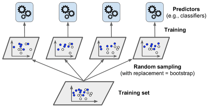
Specifically, given a training data set $D=(x_i, y_i)_i^n$ of the size $N$, we build an ensemble model of size $m$ according to the following steps:
-
For $i=1, 2, 3, …, m$
- draw $N'(N' \le N)$ samples with replacement from $D$, which is denoted by $D^*_i$
- build a model (e.g. decision tree) $T^*_i$ based on $D_i^*$
-
For an unseen data, aggregate the predictions of all $T^*$
- perform a majority vote for classification
- average the predictions for regression
from sklearn.ensemble import BaggingClassifier
from sklearn.tree import DecisionTreeClassifier

ensemble_clf = BaggingClassifier(DecisionTreeClassifier(), n_estimators=300, max_sample=100, bootstrap=True)
Random Forest
Bagging can be used for any models. Among them random forest is the special one. As its name suggests, it is exclusively designed for decision trees. Besides, it introduces extra randomness when growing trees.
![Figure 3: A random subset of features at each split for each tree (Reference [2])](/blog/post/images/random-forest.jpeg)
Specifically, it randomly choose a subset of $m'$ of the features at each split instead of using all features shown in Figure 3. By doing so, all trees can have much different training data set further, so they are less similar to each other, which results in more significant predictions.
from sklearn.ensemble import RandomForestClassifier, BaggingClassifier
from sklearn.tree import DecisionTreeClassifier

random_forest_clf = BaggingClassifier(splitter='random', DecisionTreeClassifier(), max_leaf_nodes=16,n_estimators=300, max_sample=100, bootstrap=True)

## is equivalent to this
random_forest_clf=RandomForestClassifier(n_estimators=300, max_leaf_nodes=16)
Extra-Trees
TODO
Why Bagging works
Take random forests as an example, each decision tree is a machine learned from a data set. Based on the theory of bias and variance, we know that the mean meachine can be expressed as $f'_m=E_D[f'(x|D)]$. Thus, $f'(x|D)$ can be interpreted as a random variable $X$, and $f'_m$ can be described as $\mu = E(X)$.
Since we have $N$ decision trees in a random forest, there are $N$ random variables $X_i$, where $\mu = E(X_i)$. We can construct a new random variable $Z = \frac{1}{n}\sum_i^nX_i$, which represents the mean of $n$ random independent variables $X_i$.
The expected value of $Z$ is given by
$$ E[Z] = E[ \frac{1}{n}\sum_i^nX_i ] =\frac{1}{n} E[\sum_i^nX_i] = \frac{1}{n} nE[X_i] = \mu $$
The variance is
$$ E[(Z - E[Z])^2] = E[(\frac{1}{n}\sum_i^nX_i - \mu)^2] = \frac{1}{n^2} E[(\sum_i^n (X_i - \mu))^2] $$
$$ = \frac{1}{n^2}E[\sum_i^n(X_i - \mu)^2 + \sum_i^n\sum_{j=1,i \ne j}^n (X_i -\mu)(X_j -\mu)] $$
Since $X_i$ is independent of $X_j$ ( $i\ne j$ ),
$$ E[\sum_i^n\sum_{j=1,i \ne j}^n (X_i -\mu)(X_j -\mu)] = 0 $$
we are left with
$$ E[(Z - E[Z])^2] = \frac{1}{n^2}E[\sum_i^n(X_i - \mu)^2] = \frac{1}{n} \sigma^2 $$
where $E[(X_i-\mu)^2]=\sigma^2$.
From the above euqation, we can see that ensemble methods reduce variances as $n$ increases when our models are uncorrelated.
On the contrary, if our models are correlated with the correlation coefficient $\rho$
$$ \rho = \frac{E[(X_i - \mu)(X_j - \mu)]} {\sqrt{\sigma^2(X_i)}\sqrt{\sigma^2(X_j)}} $$
The variance is
$$ E[(Z - E[Z])^2] = \frac{1}{n} \sigma^2 + \frac{n-1}{n} \rho \sigma^2 = \rho \sigma^2 + \frac{(1 - \rho)}{n} \sigma^2 $$
As $n$ increases, the second term vanishes and we are left with the first term. Therefore, if we want the ensemble methods to do well, we need our models to be uncorrelated.
Random forests do a good job because of both the randomness of training data sets sampled via bootstrapping and the randomness of features considered at each split. The algorithm results in much less correlated trees, which trades a higher bias for a lower variance, generally yielding better results.
Feature Importance
Like decision tree, random forests can tell us the relative importance of each feature. It is measured by calculating the sum of the reduction in impurity over all the nodes that are split on that feature.
random_forest_clf.feature_importances_
Boosting
In boosting, we combine a group of weak learners into a strong learner.
What’s the weak learners? They are the learning machines that do a little better than chance. Thus, they have high bias but low variance. The goal of boosting is to reduce the bias by combining them.
How to construct a weak learner? Well, one of the widely used types of weak learner are very shallow trees, for example, the stump with only one depth.
AdaBoost and GradientBoost are two popular algorithms for boosting. Let’s lookt at AdaBoost first.
AdaBoost
AdaBoost is a classic algorithm for binary classification. Suppose we have a data set $D=(x^i,y^i)_i^N$ with $y^i \in {-1, 1}$, and our weak learner $h(x)$ provides a prediction $h(x^i) \in {-1, 1 }$. The goal of AdaBoost is to construct a strong learner by combining all the weak learners, which can be written as a weighted sum of weak learners,
$$ C_n(x) = \sum_i \alpha_i h_i(x) $$
How to find $\alpha_i$ and $h_i(x)$? Well, it’s difficult to find all the coefficients for one time, so we will solve this equation greedily,
$$ C_n(x) = C_{n-1}(x) + \alpha_n h_n(x) $$
where $C_{n-1}(x)$ is the current ensemble model that fit the training data best and $h_n(x)$ is the weak learner we are going to add.
Exponential Loss
The second step is to find an appropriate loss function to optimize. How do we measure the performance of a classification model? One of the most widely used loss functions is 0-1 loss,
$$ L = \sum_i^N [y_i \ne y'_i] $$
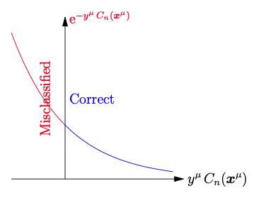
where $[y_i \ne y'_i] = 1$ if $x_i$ is classified incorrectly and 0 otherwise. However, it’s not-convex and difficult to optimize shown in Figure 4. In AdaBoost, we use exponential loss.
$$ L = \sum_i^n e^{-y^iC_n(x^i)} $$
From Figure 4, it can be seen that data that are classified correctly have lower value while misclassfication observations have much larger values, which means exponential loss punishes examples classified incorrecly much more than correct classifications.
Intuition
To minimize the loss, we plug the previous $C_n(x)$ into the loss function
$$ L = \sum_i^n e^{-y^i (C_{n-1}(x^i) + \alpha_n h_n(x^i))} = \sum_i^n e^{-y^i C_{n-1}(x^i)} e^{-y^i \alpha_n h_n(x^i)} =\sum_{y^i\ne h_n(x^i)}^n w_n^i e^{\alpha_n} + \sum_{y^i= h_n(x^i) }^n w_n^i e^{-\alpha_n} $$
$$ = \sum_{y^i= h_n(x^i) }^n w_n^i e^{-\alpha_n} + \sum_{y^i\ne h_n(x^i) }^n w_n^i e^{-\alpha_n} - \sum_{y^i\ne h_n(x^i) }^n w_n^i e^{-\alpha_n} + \sum_{y^i\ne h_n(x^i)}^n w_n^i e^{\alpha_n} $$
$$ = e^{-\alpha_n} \sum_i^n w_n^i + (e^{\alpha_n} - e^{-\alpha_n}) \sum_{y^i\ne h_n(x^i) }^n w_n^i $$
Then we find that minimizing the loss is equivalent to minimizing the sum of weights of each data that $h_n(x)$ misclassified, and that the value of weights depend on the current ensemble model $C_{n-1}(x)$.
$$ \sum_{y^i\ne h_n(x^i) }^n w_n^i = \sum_{y^i\ne h_n(x^i) }^n e^{-y^i C_{n-1}(x^i)} $$
- If the data misclassified by $C_{n-1}(x)$ are still classified incorrectly by $h_n(x)$, then $w_n^i$ is extremely large.
- If the data classified correcly by $C_{n-1}(x)$ are misclassified by $h_n(x)$, then $w_n^i$ is small.
Simply put, misclassified data points will get high weights while correctly classified data points will get their weights decreased.
Therefore, we are finding some weak learner that tries to correct the errors the previous learners made. Furthermore, we also notice that we need to update $w_n^i$ for the next weak learner $h_{n+1}(x)$,
$$ w_{n+1}^i = e^{-y^i C_{n}(x^i)} = e^{-y^i (C_{n-1}(x^i) + \alpha_nh_n(x^i))} = w_n^i e^{-y^i\alpha_nh_n(x^i)} $$
So the new weight of each data depends on the last weight of that data, the weight of the previous weak learner $h_n(x)$ and itself. But wait, what’s the initial weight of each data? We simply initialize weights $w_1^i = \frac{1}{N}$ for every training sample.
Okay, now we are only left with $\alpha_n$. To find $\alpha_n$, we take the derivative of $L$ with respect to $\alpha_n$
$$ \frac{\partial L}{\partial \alpha_n} = e^{\alpha_n} \sum_{y^i\ne h_n(x^i)}^n w_n^i - e^{-\alpha_n} \sum_{y^i= h_n(x^i) }^n w_n^i $$
That is
$$ \alpha_n = \frac{1}{2} In\frac{\sum_{y^i= h_n(x^i) }^n w_n^i}{\sum_{y^i\ne h_n(x^i) }^n w_n^i} $$
Algorithm
Let’s put it all together. The algorithm of AdaBoost can be summarised as below,
-
Given a data set $D=(x^i,y^i)_i^N$ with $y^i \in \{-1, 1\}$ and a group of weak learners $h(x)$ of size $T$
-
Associate a weight $w_1^i = \frac{1}{N}$ with every data point $(x^i, y^i)$
-
For $t = 1$ to $T$
- Train a weak learner $h_t(x)$ that minimises $\sum_{y^i\ne h_t(x^i) }^n w_t^i $
- Update the weight of this learner, $\alpha_t = \frac{1}{2} In\frac{\sum_{y^i= h_t(x^i) }^n w_t^i}{\sum_{y^i\ne h_t(x^i) }^n w_t^i}$
- Update weights for each training point, $w_{t+1}^i = w_t^i e^{-y^i\alpha_th_t(x^i)}$
-
Make a prediction
- $C_n(x) = sign[\sum_t^T \alpha_t h_t(x)]$
Example
Step 1: Initialisation
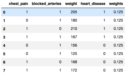
Here we have 8 rows with 3 predictors chest_pain, blocked_arteries and weight and 1 target variable heart_disease. Each data point is initialised with an equal weight 0.125.
Step 2: Find the weak learner
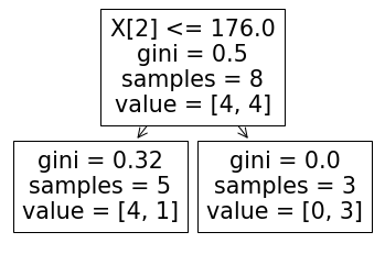
Here, we use stump as our weak learner and Figure 6 shows the first optimal tree where we only misclassified one observation.
from sklearn import tree

X = df.drop(['heart_disease', 'weights'], axis=1)
y = df['heart_disease']

clf = tree.DecisionTreeClassifier(max_depth=1)
clf = clf.fit(X, y)

tree.plot_tree(clf.fit(X, y))
plt.show()
Step 3: Update weights
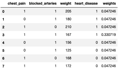
Since we have only one misclassification, the error rate is 1/8 and $\alpha_1$ is 0.97. Then we update weights for each data point using $\alpha_1$.
def cal_alpha(error):
    return 0.5*np.log((1 - error)/error)

alpha_1 = cal_alpha(1/8)

correct_samples = df[clf.predict(X) == y]
df.loc[clf.predict(X) == y, 'weights'] = correct_samples['weights'] * np.exp(-alpha_1)

misclassified_samples = df[clf.predict(X) != y]
df.loc[clf.predict(X) != y, 'weights'] = misclassified_samples['weights'] * np.exp(alpha_1)

print(alpha_1, df)
Step 4: Go back to Step 2 until the desired number of learners is reached.
Adjusted impurity
Recall that Gini Index is written as
$$ Q_m^g(L) = 1 - \sum_{c \in C } p_c(L)^2 $$
and entropy discussed in Decision Tree as
$$ Q_m^e(L) = -p_c(L)logp_c(L) $$
where $p_c(L)$ is the fraction of the observations belong to class $c$. In order to use the weight of each data in AdaBoost, we need to change it slightly.
$$ p_c(L) = \frac{\sum_{x^j \in C} w_n^j I[y_j == C]}{\sum_{x^i \in L} w_n^i} $$
Why this works? Remember that the lower the impurity is, the better the split is. And a higher fraction leads to a lower impurity or entropy.
- If we classify the misclassified example in the node $L$ correctly, then the denominator of $p_c(L)$ becomes smaller and then $p_c(L)$ becomes larger.
- On the contratry, if this split works so bad, then we will have many observations that classified incorrectly, resulting in smaller $p_c(L)$ due to a small numerator and large denominator.
Thus, we are finding the best split that can correctly classify the examples that previous learners failed as much as possible.
References
[1] A. Géron, Hands-on machine learning with Scikit-Learn and TensorFlow. Sebastopol (CA): O’Reilly Media, 2019.
[2] T. Yiu, “Understanding random forest - towards data science,” Towards Data Science, 12-Jun-2019. [Online]. Available: https://towardsdatascience.com/understanding-random-forest-58381e0602d2. [Accessed: 23-Apr-2021].
[3] J. Rocca, “Ensemble methods: bagging, boosting and stacking - Towards Data Science,” Towards Data Science, 23-Apr-2019. [Online]. Available: https://towardsdatascience.com/ensemble-methods-bagging-boosting-and-stacking-c9214a10a205. [Accessed: 23-Apr-2021].
[4] Gradient Boosting Tutorial http://talks.albertauyeung.com/pycon2017-gradient-boosting/