Information Theory
I remembered that I learned a little stuff about information when I was in my undergraduate course. Well, maybe I was wrong. It’s been almost ten years. But when it comes to information theory, I know that we will talk about a person — Shannon. So what’s the information theory? What problems does it help to solve?
Information
First, let’s understand what information is. Consider a guessing game where Alice randomly chooses a number between 1 and 100, and then we need to guess what that number is. An intuitive method is to use a dichotomy search. We may ask, ‘is it larger or smaller than 50?’. If it’s less than 50, we continue to ask, ‘is it larger or smaller than 25?’ We do this iteratively until we find the right number. Mathematically, the number of searches is $log_2(100)$. If the number Alice chooses is small, say 3, then it would take many steps to get the correct answer.
If we know that Alice has some preferences for some particular numbers, say she likes 88 most. Then the first question we ask at this time would be ‘is it 88?’. If we are lucky enough, we will get the number once. On the other hand, since 88 is the number that Alice likes most, there is no doubt that she is likely to choose 88 as the riddle. Conversely, if Alice is going to surprise us, she would choose a number that she doesn’t like very much. If so, it increases the uncertainty of our guess, i.e. we would need to ask more questions.
The number of questions we ask or the degree of surprise is information, which is measured by
$$ I(X=x) = -\text{log}P(X=x) $$
where $P(x)$ is a probability of occurence of x. When using the natural logarithm, the information unit is nat. One nat is the amount of infomration gained from the event with the probability of $\frac{1}{e}$. Besides, we also use bit as the unit if the log base is 2.
In short, information quantifies how uncertain an event is. A rare event will cause much surprise and consequently contain much information.
Entropy
Suppose we have a probability distribution $P(x)$ over a random variable $X$, and the value of each outcome represents information associated with it. The entropy of $X$ is then defined as the expectation of information,
$$ H(X) = -\sum_{x \in X} P(X=x) \text{log} P(X=x) $$
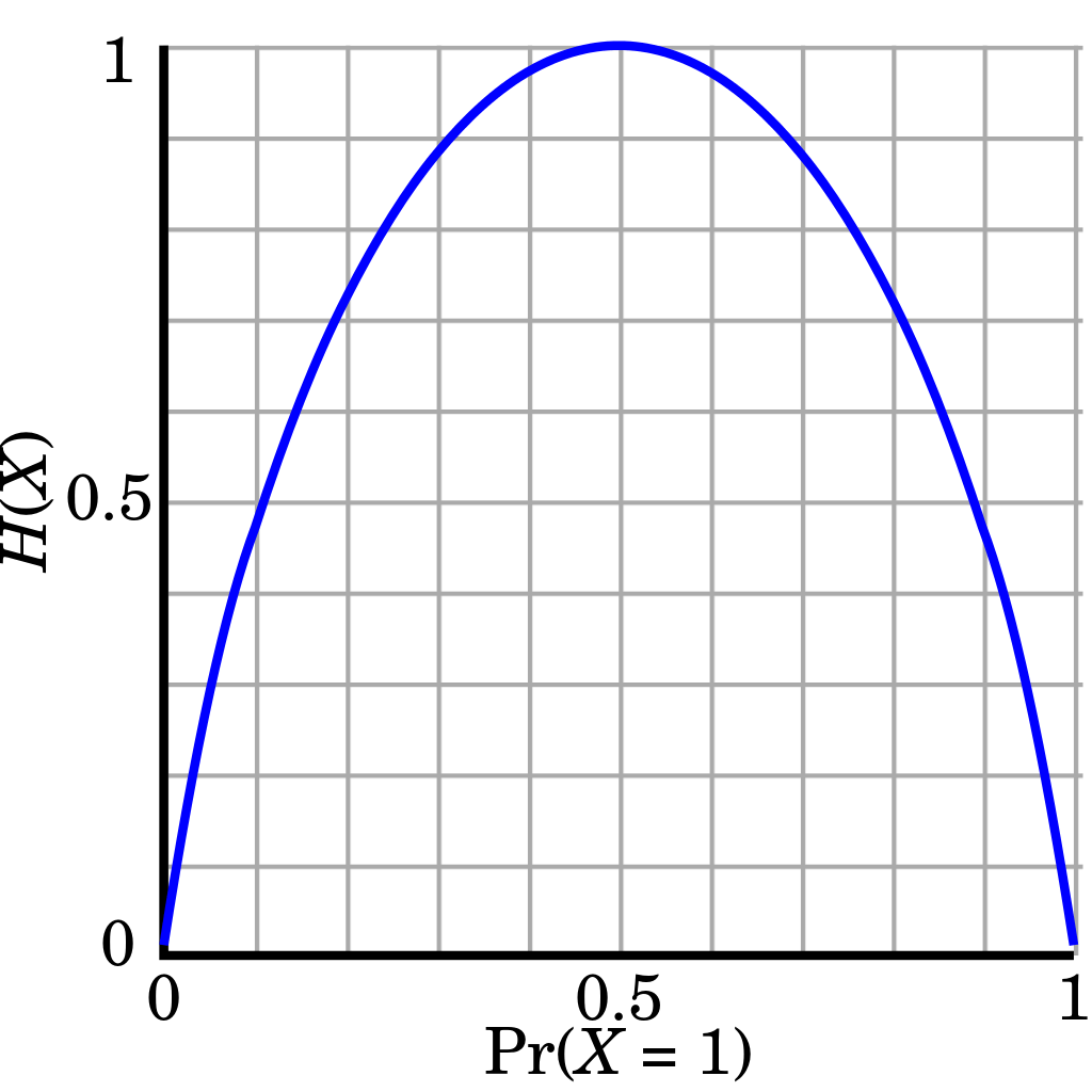
If a random variable $X$ follows binominal distribution with probability $p$, then its entropy is computed as follows,
$$ H(X) = -p\text{In}p - (1-p)\text{In}(1-p) $$

Figure 1 shows how $H(X)$ changes as $p$ changes. We can see that $H(X)$ tends to be zero if $p$ lies on the end of x-axis, which means that it tells us rare information since we know what to expect. On the contrary, $H(X)$ reaches the highest point if $p=0.5$, this is because we don’t know what to expect and anything could happen. From this view, entropy is also a measure of how uncertain $X$ is. The higher the entropy is, the higher the uncertainty is.
KL Divergence
Given two probability distribution $f(x)$ and $g(x)$ for a random variable $x$, the difference between them is defined as KL divergence, which is sometimes called relative entropy
$$ D(f||g) = \sum_{x \in X} f(x) \text{log} \frac{f(x)}{g(x)} = -\sum_{x \in X} f(x) \text{log} g(x) + f(x) \text{log} f(x) $$
Cross-entropy
Combing the definition of entropy, we have
$$ H(f)= -\sum_{x \in X} f(x) \text{log} f(x) $$
$$ H(f, g) = -\sum_{x \in X} f(x) \text{log} g(x) $$
$$ D(f||g) = H(f, g) - H(f) $$
where $H(f, g)$ is cross-entropy, which is the expected information of $X$ sampled from a probability distribution $f(x)$ with outcomes encoded using another distribution $g(x)$. We can find that KL divergence can be decomposed into two parts: cross-entropy and the entropy of $X$ sampled from $f(x)$. Usually $f(x)$ is considered as ‘true’ probability distribution, so miniming KL divergence against a fixed reference distribution $f$ is equivalent to minimising cross-entropy.
Cross-entropy is a common loss function used in classification tasks. Suppose there are 3 classes, the class distribution for a given $x$ is $0, 1, 0$ and our model might give us a predicted class distribution, say $0.2, 0.5, 0.3$. Then, we calculate entropy for this observation, $H(f, g) = -(0 + 1 *\text{log}0.5 + 0) = 1$. After a period of learning, the model could give us a better predicted label distribution say $0.05,0.9,0.05$, and this time, we find that the entropy decreases to $0.15$. It shows that the difference between our model and true distribution is decreasing.
Conditional Entropy
Like conditional probability, we define conditional entropy as the uncertainty about a random variable $C$ after we observe one feature $x$ in $X$
$$ H(C|X=x) = -\sum_{c \in C} p(c|X=x) \text{log} p(c|X=x) $$
The difference between the entropy $H(C)$ and the conditional entropy $H(C|X=x)$ is realized information
$$ I[C; X=x] = H(C) - H(C|X=x) $$
Hence, $I(C;X=x)$ measures how much uncertainty of $C$ changes due to observering $x$. Here, we use ‘change’ because realized information is not always reduced.
Mutual Information
Mutual information defined below tells us the expected reduction in uncertainty of $C$ that a feature gives us
$$ I(C; X) = H(C) - \sum_x p(X=x) H(C|X=x) $$ Here are some important notes about mutual information:
- it is always positive
- it is zero if $C$ and $X$ are statistically independent
- it is symmetric in X and C
In fact, we have met mutual information before — information gain in decision trees.