Linear Regression 01
There are two main tasks in machine learning: regression and classification. Today we will talk about regression, more specifically, linear regression. Linear regression is simple and easy to understand. Perhaps it is the first algorithm that most people learn in machine learning. So let’s go!
Problem Statement
Suppose you are a teacher, and you recorded some data about the hours students spent on study and the grades they achieved. Below are some sample data you collected. Then you want to predict the score for someone according to the hours he spent.
| Hours | 0.5 | 1 | 2 | 3 | 4 |
|---|---|---|---|---|---|
| Grade | 20 | 21 | 22 | 24 | 25 |
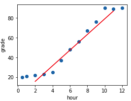
How to make a prediction? Since there are only two variables, let’s plot them to see if there is a relation betwee grade and hours.

Figure 1 shows that grade is positively related to hours. For simplicity, we can use a straight line(the red line) to approximate this relation. And this is exactly our first linear model.
Simple Linear Regression
Remember the equation of a straight line is typically written as,
$$ y = ax + b $$
In this example, $x$ is the variable hours and $y$ is the variable grade, which we’ve already known. So the problem is to find the parameter $a, b$ such that the red line is as close as possible to the blue data points. Technically, this is called parameter estimation. Usually, there are two ways to do this: minimising the loss and maximising the likelihood. Now we focus on the former.
Residual
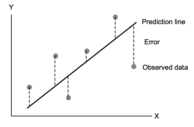
So how to measure the closeness mentioned above? The most common way is to measure the residual, which is the difference between the estimated value and our true value shown in Figure 2. For a single data point, the residual is defined as below, where $y_i$ is the true value and $y_i'$ is our predicted value.
$$ e = y_i - y'_i = y_i - ax_i - b $$

error
Since we have many data points, we need to sum them up to evaluate the overall errors. Unfortunately, some error terms will cancel out when you do the this calculation directly.
$$ L = \sum_i^n (y_i - y'_i) = \sum_i^n (y_i - ax_i - b) $$
the absolute value of error
One way to tackle this is to take the absolute value of the error terms. However, the absoulte value of $x$ is not differentiable at $0$.
$$ L = \sum_i^n |y_i - y_i'| $$
the squared value of error
Instead of taking the absolute value, we square all the errors and sum them up, which is known as the Residual Sum of Squares(RSS) or Sum of Squared Error (SSE).
$$ L = \sum_i^n (y_i - y_i')^2 $$
Closed-form solution
Finally, we find a function to measure the loss. Next, we need to find the parameters that minimize the squared error. The good news is that our loss function is differentiable and convex! It means that we have the global minimum value and can be calculated directly by taking derivatives.
Let’s take the first derivative w.r.t $b$
$$ \frac{\partial L}{\partial b} = \sum_i^n -2(y_i - ax_i-b) $$
and then set this equation to $0$,
$$ -2(\sum_i^ny_i -a\sum_i^nx_i - \sum_i^nb) = -2(n\overline y-an\overline x - nb) = 0 $$
$$ \hat b = \overline y - \hat a \overline x $$
Similarly, let’s take the first derivative w.r.t $a$
$$ \frac{\partial L}{\partial a} = \sum_i^n -2x_i(y_i - ax_i-b) $$
plug $b$ into this equaiton and set this equation to 0 again,
$$ \sum_i^n -2x_i(y_i - ax_i-\overline y+a\overline x) = \sum_i^n -2x_i[(y_i-\overline y)- a(x_i -\overline x)] $$
$$ \hat a = \frac{\sum_i^nx_i(y_i-\overline y)}{\sum_i^nx_i(x_i -\overline x)} $$
Here, we use a slight algebra trick,
$$ c\sum_i^n(x_i - \overline x_i) = 0 $$
plug the above equation into the previous equation
$$ \hat a = \frac{\sum_i^nx_i(y_i-\overline y)}{\sum_i^nx_i(x_i -\overline x)} = \frac{\sum_i^nx_i(y_i-\overline y) - \sum_i^n\overline x(y_i - \overline y)}{\sum_i^nx_i(x_i -\overline x) - \sum_i^n\overline x(x_i - \overline x)} $$
$$ = \frac{\sum_i^n(x_i-\overline x)(y_i-\overline y)}{\sum_i^n(x_i -\overline x)^2} $$
$$ = \frac{Cov(x, y)}{Var(x)} $$
Finally, we find the best estimators for our simple linear regression.
Test statistics
The above formulas give us the best estimation for the parameters $a, b$ of the linear regression model. If we generate different data sets from the population, we will have different linear models and different values of dependent variable. If we average these values, we’ll find that the average value is pretty close to the true value. Mathematically, this can be expressed as follows,
$$ E_D(\hat ax_i + \hat b|D) \simeq ax_i+b $$
The idea behind the above equation is analogous to the Central Limit Theorem for Sample Mean. The population mean of the random variable $Y_i$ (the true line) can be estimated by the expected value of the sample mean(the estimated line). CLT tells us the distribution of the sample mean follows the Gaussian Distribution with the mean of the population mean as the sample size gets larger.
Standard error
But in practice, we can only have one data set, so how accurate is the parameters $a, b$ calculated from the above equations? In other words, a single sample mean may overestimate or underestimate the population mean, but to what extent is this deviation? We use the standard error of sample mean to measure it, which can be obtained by the following equation, where $\sigma$ is the population standard deviation and $n$ is the sample size.
$$ SE^2(\hat {\overline \mu}) = Var(\hat {\overline \mu}) = \frac{\sigma^2}{n} $$
Similarly, we can calculate the standard error associated with the parameters $a$ and $b$.
$$ SE^2(\hat a) = Var(\frac{\sum_i^n(x_i-\overline x)(y_i-\overline y)}{\sum_i^n(x_i -\overline x)^2}) = Var(\frac{\sum_i^n(x_i-\overline x)y_i - \sum_i^n(x_i-\overline x)\overline y}{\sum_i^n(x_i -\overline x)^2}) $$
$$ = Var(\frac{\sum_i^n(x_i-\overline x)(ax_i + b + \epsilon_i)}{\sum_i^n(x_i -\overline x)^2}) $$
$$ = \frac{\sum_i^n(x_i-\overline x)^2}{(\sum_i^n(x_i -\overline x)^2)^2} Var(ax_i + b + \epsilon_i) = \frac{\sum_i^n(x_i-\overline x)^2}{(\sum_i^n(x_i -\overline x)^2)^2} Var(\epsilon_i) $$
$$ = \frac{Var(\epsilon_i)}{\sum_i^n(x_i -\overline x)^2} $$
Since $x_i, y_i$ are known and $a, b$ are the true parameters, the only thing unknown is $\epsilon_i$. In other words, they are all indepentdent of $\epsilon_i$. In addition, we use a bit tricks to derive the above formula,
$$ Var(c) = 0 $$
$$ Var(cX) = c^2Var(X) $$
$$ Var(c + X) = Var(X) $$
In summary, what we should know is that the standard error of $\hat a$ tells us how far away this estimate $\hat a$ is from the true value $a$ or how far away the predicated value $\hat y$ is from the observed value $y$.
Furthermore, since the predicted value obtained from a given sample is different from the true value, we cannot say we are sure that the estimated value is exactly the true value. But we could say we are 90% confident that the true value lies somewhere around the predicted value. And this ‘somewhere’ can be computed by confident intervals.
p-value
To investigate whether the estimated parameters are statistically significant, we perform hypothesis tests. A statistical significant result means it’s unlikely to happen by chance. In the simple linear regression, the null and alternative hypotheses are defined as
$H_0$: There is no relationship between $X$ and $Y$
$H_a$: There is some relationship between $X$ and $Y$
Mathematically, it is equvalent to testing
$H_0$: $a=0$
$H_a$: $a\ne0$
So in order to test the null hypothesis, we need to demonstrate that $\hat a$ is sufficiently far away from $0$. Thus, we can be confident that $a$ is not equal to $0$ and reject the null hypothesis. To quantify the distance between $\hat a$ and $0$, we calculate t-score
$$ t = \frac{\hat a - 0}{SE(\hat a)} $$
The higher the $t$ is, the farther the distance is. But wait, what’s the probability of getting this estimate $\hat a$ or more extreme? In other words, what’s the p-value? How to interpret this probability? A higher p-value doesn’t provide much information. In contrast, a smaller p-value means it’s unlikely to observe this t-score due to chance under the assumption that $H_0$ is true. You can interpret that a small p-value indicates a strong evidence against the null hypothesis. But how small is enough? Typically, we set the threshold value of $0.05$. If p-value is smaller than $0.05$, we reject $H_0$, otherwise we accept it.
Model Evaluation
Next question is how to evaluate our model? How good is it? There are two common metrics to measure the quality of a linear regression model: RSE and $R^2$.
RSE
Residual standard error measures the average deviation between the estimated value and the true value. It can be calculated using the following fomula, where n-2 is the degree of freedom(df) of the residual.
Q: Why do we divide by $n-2$ not $n$?
A: This is because the latter tends to underestimate variance. Rememer we divide by $n-1$ when calculating the sample variance. This is the same reason here.
Q: But why n-2?
A: We know that 2 points determine a line, which means there is no other line fitting the data and the residual of each data point is fixed. If we add a third point, there could be many lines fitting these points and thus different residuals. That means the third point increases the flexiblity of the value of residuals. We say we have one free observation. Therefore, the degree of freedom of the residual is $n-2$ in simple linear regression.
$$ RSE = \sqrt{\frac{1}{n-2} RSS} = \sqrt{\frac{1}{n-2} \sum_{i=1}^n (y_i - y_i')^2} $$
A smaller RSE indicates that our model fit the data well. However, RSE is measured in the unit of $Y$. For some data sets, RSE would be small, e.g $3.2$. But for other data sets, it would be very large, e.g $1200$. So it’s a bit confusing. That’s why $R^2$ comes. $R^2$ measures the fraction of variance explained, which is independent of the unit of $Y$.
$R^2$
Coefficient of determination or $R^2$ is another metric to measure the goodness of a linear regression model. Let’s rewrite the previous equation by multiplying both the denominator and numerator by $\sqrt {\sum_i^n(y_i-\overline y)^2}$
$$ a = \frac{\sum_i^n (x_i - \overline x)(y_i - \overline y) \sqrt {\sum_i^n(y_i-\overline y)^2}}{\sqrt {\sum_i^n(x_i-\overline x)^2} \sqrt {\sum_i^n(x_i-\overline x)^2} \sqrt {\sum_i^n(y_i-\overline y)^2}} $$
$$ a = R\frac{s_y}{s_x} $$
where
$$ R = \frac{Cov(x, y)}{\sqrt{var(x)} \sqrt{var(y)}} $$
$$ s_y = \sqrt{Var(y)} $$
$$ s_x = \sqrt{Var(x)} $$
Remember that the error is defined as $e_i = y_i' - y_i$, so the mean of $e$ is
$$ E(e) = \frac{1}{N} \sum_i^n e_i = \frac{1}{N} \sum_i^n b + ax_i - y_i =b + a\overline x - \overline y = 0 $$
and the variance is
$$ var(e) = \sum_i^n (e_i - \overline e)^2 = \sum_i^n (y_i - b - ax_i)^2 = \sum_i^n (y_i - \overline y + a\overline x - ax_i)^2 $$
Let’s plug $a$ into this equation
$$ var(e) = \sum_i^n [(y_i - \overline y) - R\frac{s_y}{s_x}( x_i - \overline x)]^2 = var(y) (1-R^2) $$
Or you might be more familiar with this equation
$$ R^2 = 1 - \frac{var(e)}{var(y)} = 1 - \frac{RSS}{TSS} $$
Therefore, $R^2$ tells us how much the variance of $y$ has been explained by our models. The higher the $R^2$ is, the better our model is.
References
[1] Bradthiessen.com, 2021. [Online]. Available: https://www.bradthiessen.com/html5/docs/ols.pdf. [Accessed: 14- Apr- 2021].
[2] “Linear Regression - ML Wiki,” Mlwiki.org. [Online]. Available: http://mlwiki.org/index.php/Linear_Regression. [Accessed: 14-Apr-2021].
[3] K. Base and S. statistics, “Standard Error | What It Is, Why It Matters, and How to Calculate”, Scribbr, 2021. [Online]. Available: https://www.scribbr.com/statistics/standard-error/. [Accessed: 12- May- 2021].