Metrics for classification
In linear regression, we choose $R^2$ as our metrics to measure how good our algorithms are. But how about classification? In this post, we are going to talk about several commonly used metrics for classification.
Metrics
We first consider the binary classification, where an example must be classified as either A or B. Thus, there are four possible cases,
- the ground truth is A, and the predicted lable is A
- the ground truth is A, but the predicted lable is B
- the ground truth is B, and the predicted lable is B
- the ground truth is B, but the predicted lable is A
Often, we use a confusion matrix to contain all these conditions, as Table 1 shows.
Confusion Matrix
| predicted\ground truth | P | N |
|---|---|---|
| P | TP | FP |
| N | FN | TN |
Based on the confusion matrix, we can derive some useful metrics to measure model performance from various aspects.
Accuracy
Accuracy tells us how well a classifier is in general by considering both positive and negative examples that are correctly classified.
$$ \text{Accuracy} = \frac{TP + TN}{ TP + FP + FN + TN} $$
The drawbacks of accuracy are obvious. When we have imbalanced data where the number of negative examples is much more than positive examples, TN tends to be dominant, making no sense in most cases. For example, the number of O is more than the number of named entities in NER, resulting 99% accuracy. However, it does not indicate our classifier works well. By contrast, it may not be able to recognize any entity at all!
Precision
Precision tells us how many true positive examples are in all predicted positive examples, which is calculated as follows,
$$ \text{ Precision } = \frac{TP}{ TP + FP} $$
From the above equation, we can see that larger TP and smaller FP will lead to higher precision. That makes sense because more examples that belong to either the class of interest or the negative are identified correctly. (PS: FP is also known as Type-1 Error.)
Spam detection is a classical binary classification. It’s fine if several spam emails are escaped from our classifier. However, if some non-spam (or ham) emails are identified as spam, that’s really a stupid decision — we would miss some important emails! Similarly, precision are more important in recommender systems, where wrong recommendation would bring bad experience to customers.
TPR/Recall
Sometimes, we would prefer to identify all cases from the actual positive classes even at a cost of lower precision. That is, we seek a higher recall (sensitiviy, TPR), which is shown below.
$$ \text { Recall } = \frac{TP}{ TP +FN } $$
For example, it does not cause much serious impacts if people who are not pregnant were diagnosed as pregnant. However, if women who are pregnant were not identified, well, you are in a big trouble. (PS: FN is also called Type-II Error.)
I’m often confused with the two metrics. Which one should I focus more on ? Precision or recall?
- FP is a higher concern, then it’s precision; otherwise, it’s recall
You can also consider in this way — whether the examples of interest are not identified (or recalled) result in little or no consequence,
- if yes, then it’s precision; otherwise, it’s recall.
One or two spam emails in our inbox is acceptable but one neglected patient with illness can cause a big flu!
Specificity
Like Recall, we can also define specificity — out of all the negative classes, how much we predicted correctly.
$$ \text { Specificity } = \frac{TN}{ FP + TN } $$
F1-Score
F1-Score is the harmonic mean of precision and recall. F1-Score is preferable if we want to balance the precision and recall.
$$ \text {F1-score} = 2 * \frac{ \text {precision} * \text {recall} }{\text {precision} + \text {recall}} $$ It is an effective metric in the following cases:
- FP and FN are equally cost
- True Negative is high
- Adding more data doesn’t effectively change the outcome
ROC-AUC
The ROC (Receiver Operator Characteristic) curve is plotted with TPR (True Positive Rate or Recall) against the FPR (False Positive Rate) at various threshold values, where TPR is on the y-axis and FPR is on the x-axis.
- A greater FPR means higher the number of FP than TN
- A smaller TPR means higher the number of FN than TP
Thus, the ROC curve depicts the trade-off between Type-I and Type-II Error. Below are code snippets of the implementation of ROC, and the plot is shown in Figure 1.
def ROC(yp1, yp2):
    pmin = np.min(np.array( (np.min(yp1), np.min(yp2)) ))
    pmax = np.max(np.array( (np.max(yp1), np.max(yp2)) ))
    print(f'min: {pmin}, max:{pmax}')

    iters = 50
    thRange = np.linspace(pmin, pmax, iters)
    ROC = np.zeros((iters, 2))
    accuracy = np.zeros(iters)

    for i in range(iters):
        threshold = thRange[i]

        # C_2 is positive while C_1 is negative, and if y > threshold, then it's positive
        TP = np.sum(yp2 > threshold) / len(yp2)
        FP = np.sum(yp1 > threshold) / len(yp1)

        ROC[i, :] = [ TP, FP ]
        accuracy[i] = np.sum(yp2 > threshold) + np.sum(yp1 < threshold)

#     auc = -1 * np.trapz(ROC[:, 0], RPC[:, 1])

    return ROC, accuracy

roc, accuracy = ROC(yp1, yp2)
fig, ax = plt.subplots(figsize=(6,6))
ax.plot(roc[:,1], roc[:,0], c='m') # FP vs TP
ax.set_xlabel('False Positive')
ax.set_ylabel('True Positive')
# ax.set_title(f'ROC curve, AUC = {auc:.2f}' )
ax.grid(True)

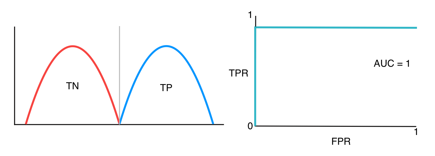
AUC (Area Under Curve) is the area under the ROC curve. The value is between 0 and 1. The greater the AUC, the better is our classifier.
-
If two classes are well separated, the auc is close to 1
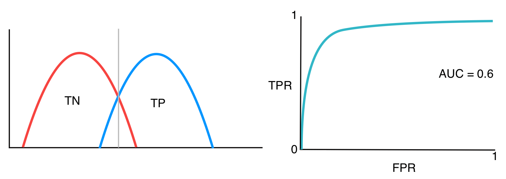
-
Usually, two classes overlap, so we get ROC like the one below
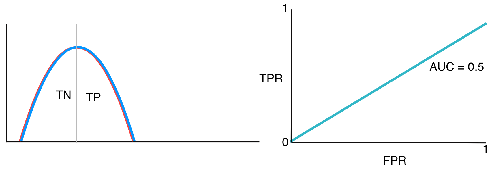
-
If they overlap further so that the AUC is approximately 0.5, our model has no ability to distinguish them
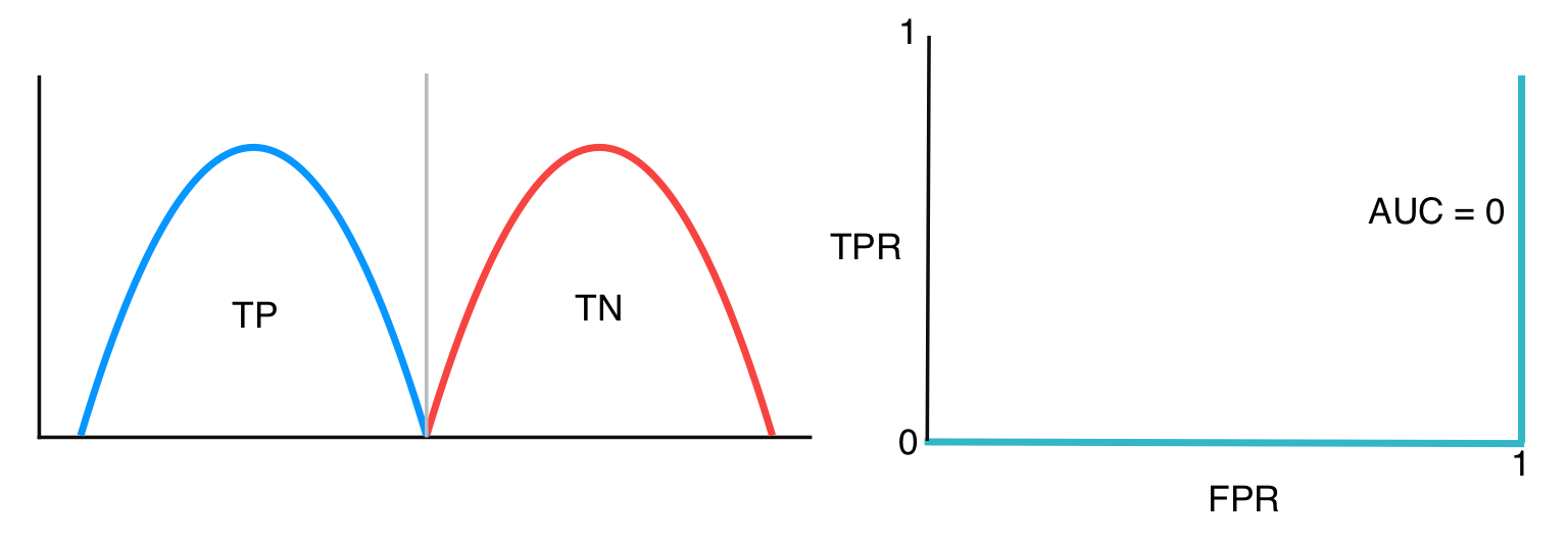
-
The worst case is that the model gives the contrary prediction as shown below
Multiclass
In the case of the multiclass classification, we have the corresponding confusion matrix for each class based on the one-vs-all methodology, as Figure 2 shows. Then, there are two choices we’re facing
- macro-averaging
- combine all classes and average them
- a more balanced overview
- micro-averaging
- pool the corresponding group from each class
- the result would be dominated by frequent classes
