Singular Value Decomposition
Singular Value Decomposition(SVD) is an important concept in Linear Algebra. Any matrix can be decomposed into the multiplication of three matrices using SVD. In machine learning, SVD is typically used to reduce dimensionality. Another popular dimension reduction technique is PCA. We will cover both of them in this post.
Change of Basis
Suppose there is a point in the 2D space, how do you describe it? The common way is to use the Cartesian coordinate system, which is composed of two fixed perpendicular oriented axes, measured in the same unit of length. The two perpendicular axes are just a special set of vectors served as the basis of the 2D space. Actually, there are many other sets of vectors that can be the basis for the 2D space. For example, in Figure 1, the position of the red point is (-4, 1) when using the standard basis (1, 0), (0, 1) (colored in grey). If we change the basis to (2, 1), (-1, 1) (colored in blue), the position is (-1, 2).

From Figure 1, we can see that the absolute position of the red point always stay the same. However, the relative positions to the different bases are different. Mathematically, the red point can be described from the perspective of basis as follows,
$$ x = P_b[x]_b = c_1 \bold b_1 + c_2 \bold b_2 + … + c_n \bold b_n $$
$$ P_b = [\bold b_1, \bold b_2, … , \bold b_n ] $$
$$ [x]_b = [c_1, c_2, … c_n] $$
where
- $[x]_b$ is a set of scalars, which represent the length of projection onto each axis of the current coordinate system
- $P_b$ is the corresponding basis of the current coordinate system
Let’s plug the above point and the basis (1, 0), (0, 1) (colored in grey) into the equation,
$$ P_b = [ (1, 0), (0, 1)] $$
$$ [x]_b = (-4, 1) $$
$$ x_b = -4 \begin{bmatrix}1\\ 0 \end{bmatrix} + 1 \begin{bmatrix}0\\ 1 \end{bmatrix} = \begin{bmatrix}-4\\ 1 \end{bmatrix} $$
Let’s do the same calculation with another basis (colored in blue),
$$ P_b = [ (2, 1), (-1, 1)] $$
$$ [x]_b = (-1, 2) $$
$$ x_b = -1 \begin{bmatrix}2\\ 1 \end{bmatrix} + 2 \begin{bmatrix}-1\\ 1 \end{bmatrix} = \begin{bmatrix}-4\\ 1 \end{bmatrix} $$
As expected, they yield the same result. And the second one essentially changes the basis of $R^2$ from (2,1),(-1,1) to(1,0),(0,1), which is the standard basis of $R^2$.
Actually, this example is a special case of the change of basis, where the new basis is the standard basis. More generally, $P_{c \larr b}$ is known as **the change of coordinate matrix from the old basis $b$ to the new basis $c$, which we are going to switch to** in $R^n$.
Say we are in the basis $b$ and $[x]_b$ is known, the corresponding coodinates of $x$ under the new basis $c$ can be computed as follows,
$$ x_c = P_{c \larr b} x_b $$
Since $P_{c \larr b}$ is invertible, we have
$$ (P_{c \larr b})^{-1}x_c = x_b $$
which is the inverse operation of change of basis from $b$ to $c$. We can generalize this to any number of points and dimensions.
$$ A=US\\(D,N)= (D, M) \times (M, N) $$
$$ U^{-1} A = S\\(M, D) \times (D, N) = (M, N) $$
where
- $A$ is a $D\times N$ matrix with $D$ dimensions and $N$ points
- $S$ is a $M\times N$ matrix with $M$ dimensions and $N$ points described in a new vector space decided by another basis
- $U$ is the change of coordinate matrix from $S$ to $A$
- $U^{-1}$ is the the change of coordinate matrix from $A$ to $S$
If we do some transformation for a point in the standard coordinate system, what’re the new coordinates of the same point in another system? This problem can be solved by the following equation,
$$ x_s' = U^{-1}TUx_s $$
where $T$ represents the transformation matrix. If $T=I$, $x_s'$ is exactly $x_s$.
SVD
SVD is a technique in linear algebra that can be used to decompose any $N \times P$ matrix
$$ X = U S V^T $$
- $U$ is an $N \times N$ orthogonal matrix, where the columns of $U$ are the eigenvectors of $XX^T$
- $S$ is an $N \times P$ diagonal matrix whose diagonal entries are the sorted singluar values, which are square roots of eigenvalues of $XX^T$ or $X^TX$
- $V$ is a $P \times P$ orthogonal matrix, where the columns of $V$ are the eigenvectors of $X^TX$
$$ C = X^TX = (USV^T )^T USV^T = VS^TU^T USV^T = VSS^TV^T $$
$$ D = XX^T = USV^T (USV^T )^T = USS^TU^T $$
$$ => C [\bold v_1, \bold v_2, …, \bold v_p] = [\lambda_1 \bold v_1, \lambda_2\bold v_2, …, \lambda_p \bold v_p] $$
$$ => D [\bold u_1, \bold u_2, …, \bold u_n] = [\lambda_1 \bold u_1, \lambda_2\bold u_2, …, \lambda_n \bold u_n] $$
Therefore, $V$ and $U$ are matrices of eigenvectors for $X^TX$ and $XX^T$.
If we look at the formula of SVD from the view of ‘the change of basis’ discussed above, we will find that
- $V^T$ is the change of matrix from, say basis A, to the standard basis
- $S$ is a scaling matrix
- $U$ is another change of matrix from the standard basis to basis A
Geometrally, the multiplication between a matrix $A$ and a vector $x$ represents a linear transformation, where we using another basis of $R^n$ to represent the same point and $A$ is the change of matrix between bases. By decomposing $A$, we can clearly see that this transformation is composed of three transformations:
- $ V^T$: rotation
- $S$: scaling
- $U$: rotation
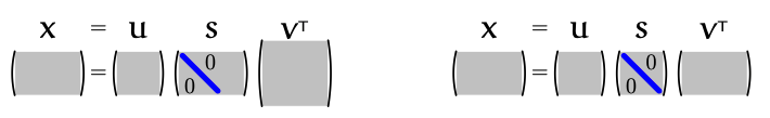
Economical Forms of SVD
Since $S$ is an $r \times r$ diagonal matrix for some $r$ not exceeding the smaller of $N$ and $P$, we could simplify $S$ and the correspoding $V$ and $U$. Specifically, for $X$ with more samples than features $N > P$ (tall and thin), we ignore the last $N - P$ columns of U
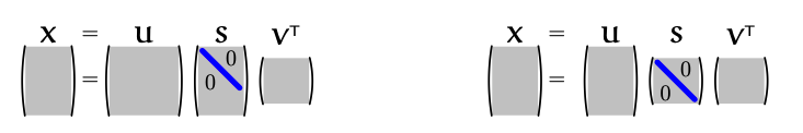
and for $X$ with more features than examples $N < P$ (short and fat), we ignore the last $P - N$ rows of $V^T$
Linear Regression Revisited
In the previous post Linear Regression 02, we introduced pseudo-inverse $A^+$
$$ \bold {\hat w} = A^+ \bold y = (\bold X^T\bold X)^{-1} \bold X^T \bold y = V (S^TS)^{-1}S^TU^T \bold y = VS^+U^T \bold y $$
where the elements of $S^+$ are the reciprocal of the singular values,
$$ S^+ = (S^TS)^{-1}S^T = \begin{bmatrix}s_1^{-1}&0 & 0 & … & 0 & 0 & 0 & … & 0\\ 0&s_2^{-1} & 0 & … & 0 & 0 & 0 & … & 0\\ … \\ 0&0 & 0 & … & s_p^{-1} & 0 & 0 & … & 0\end{bmatrix} $$
This means if any of the singular values of $X$ are small, then $S^{-1}$ will magnify component in that direction. Thus, little change in $\bold y$ will lead to a greatly different model and eventually a poor generalization.
One way to tackle this is regularisation. Ridge Regression is one variant of linear regression by adding a regulariser $\lambda ||\bold w||^2$ to the loss function,
$$ L = ||\bold X \bold w - \bold y||^2 + \lambda ||\bold w||^2 $$
The estimate $\bold w$ is given by
$$ \bold {\hat w} = V(S^TS + \lambda I)^{-1} S^TU^T \bold y $$
where
$$ (S^TS + \lambda I)^{-1} S^T = \begin{bmatrix}\frac{s_1}{s_1^2+\lambda}&0 & 0 & … & 0 & 0 & 0 & … & 0\\ 0&\frac{s_2}{s_2^2+\lambda} & 0 & … & 0 & 0 & 0 & … & 0\\ … \\ 0&0 & 0 & … & \frac{s_p}{s_p^2+\lambda} & 0 & 0 & … & 0\end{bmatrix} $$
- if $s_i = 0$, then $\frac{s_i}{s_i^2 + \lambda} =0$ and the ‘inverse’ is defined
- if $s_i « \lambda$, then $\frac{s_i}{s_i^2 + \lambda} \simeq \frac{1}{\lambda }$
- if $si » \lambda$, then $\frac{s_i}{s_i^2 + \lambda}\simeq s_i^{-1}$
Therefore, adding a regulariser can make our model much more stable.
PCA
Principal component analysis(PCA) is often used to reduce dimentionality. The idea of PCA is to find directions along which data has the largest variation. The variation can be computed by projecting data onto that direction. Mathematically, we want to find a vector $v$ with $||v||=1$ to maximise
$$ \sigma^2 = \frac{1}{n-1}\sum_i^n(\bold v^T (\bold x_i - \bold \mu))^2 $$
There are two things to notice here:
- $v$ is an unit vector since we are care about the direction only
- data are centralized first for simple computation; centralizing data doesn’t change the distribution of data
We can solve the above equation by introducing Lagrange multiplier
$$ L = \frac{1}{n-1}\sum_i^n(\bold v^T (\bold x_i - \bold \mu))^2 - \lambda (||v||^2 - 1) $$
$$ = \frac{1}{n-1}\sum_i^n \bold v^T (\bold x_i - \bold \mu)(\bold x_i - \bold \mu)^T\bold v - \lambda (||v||^2 - 1) $$
$$ = \bold v^T \bold C \bold v - \lambda (\bold v^T\bold v - 1) $$
where $\bold C$ is the covariance matrix of $X$. Then we take the derivative of $L$ w.r.t $\bold v$ , and then set it to $0$
$$ \frac{\partial L}{\partial \bold v} = 2(C \bold v - \lambda \bold v) = 0 $$
so $\bold v$ is the eigenvector of $\bold C$, and the variance along this direction is,
$$ \sigma^2 = \frac{1}{n-1}\sum_i^n(\bold v^T (\bold x_i - \bold \mu))^2 = \bold v^T \bold C \bold v = \lambda \bold v^T \bold v = \lambda $$
Properties of Covariance Matrix
We know that the quadratic form of a vector and a matrix is defined as
$$ x^T M x $$
Thus, the quadratic form of $C$ is
$$ x^TCx = x^T XX^Tx=u^Tu \ge 0 $$
so $C$ is positive semi-definite, which means all eigenvalues of $C$ are greater than or equal to zero. Why? Suppose $\mu$ is an eigenvector of $C$, since $\mu^TC\mu\ge0$ and $||\mu||>0$, then we have
$$ \mu^TC\mu = \mu^T \lambda \mu => \lambda = \frac{\mu^TC\mu }{||\mu||^2 } \ge 0 $$
zero eigenvalue
What if $C$ has a zero eigenvalue? Well, a zero eigenvalue means that there is no variation in the direction of the corresponding eigenvector. So when will we have zero eigenvalues? Based on the definition of eigenvalue, we have
$$ Cx = 0x = 0 $$
Since $x$ is nonzero vector, $C$ is singular or non-invertible. And this will inevitably happen if the number of features is much more than the number of examples. Conversely, if $C$ is invertible, it has no zero eigenvalues and is said to be positive definite (since all eigenvalues are greater than 0).
Geometry of PCA
Since $C$ is a $p \times p$ symmetric matrix, it can be orthogonally diagonalized as $C = PDP^T$, where $P$ is an orthogonal matrix and $D$ is a diagonal matrix. Thus, the above formula can also be written as follows,
$$ \sum_i^n(\bold v^T (\bold x_i - \bold \mu))^2 = \sum_i^n \bold v^T (\bold x_i - \bold \mu)(\bold x_i - \bold \mu)^T\bold v = \bold v^T C \bold v $$
$$ = \bold v^T PDP^T \bold v = \bold y^T D \bold y $$
where $\bold y = P^T \bold v$. Mathematically, $\bold v^T C \bold v$ and $\bold y^T D \bold y$ yield the same result, which represents the sum of deviation of each sample from the original point along the direction determined by this vector as shown in Figure 2.
")
Geometrically, $P^T_{y \larr v}$ is the change coordinate matrix from $v$ to $y$, which finally transform the shape of the quadratic form $\bold v^TC\bold v$ into the standard position, such as the shapes in the figure below.
")
Projection
For a data set with $p$ features, we want to reduce its dimension to $k$, there are a few steps to follow
-
Construct a $p\times p$ covariance matrix $C$ using centralized data
-
Find all the eigenvectors $v_i$ and eigenvalues $\lambda_i$ of $C$
-
Construct a $p \times k$ projection matrix $P$ with $k$ eigenvectors determined by the $k$ largest eigenvalues (principal components)
-
Project the original data into the space spanned by the principal components
$$ \bold z = P^T(\bold x - \bold \mu) $$
where $\bold z$ is our new inputs.
Usually, there are two common ways to find the eigenvalues:
- eigendecomposition
- SVD
Eigen-decomposition follows the above steps, and we can see it from the following code,
def pca(X):
    # Data matrix X, assumes 0-centered
    P, N = X.shape

    # Compute covariance matrix, where X is a P by N matrix
    C = np.dot(X, X.T) / (N-1)

    # Eigen decomposition
    eigen_vals, eigen_vecs = np.linalg.eig(C)

    # Project X onto eigen space
    X_pca = np.dot(eigen_vecs.T, X)

    return X_pca, eigen_vals, eigen_vecs
Instead, SVD decomposes $X$ directly. Besides, we don’t need to centralize data first in SVD, though most people will do.
def svd(X):
  N, P = X.shape

  # In practice, we usually subtract the mean from data and then perform SVD
  X_c = X - np.mean(X, axis=0)

	# the columns of Vt are the eigenvalues of X^TX
  U, Sigma, Vt = np.linalg.svd(X_c)

	# Project X onto eigen space
  X_pca = np.dot(X, Vt.T)

  return U, Sigma, Vt
So why do we use SVD? Simply put, If the number of features are much more than the number of example, i.e. $P»N$, it’s not easy to compute eigenvalues using eigen-decomposition. But in SVD, the algorithm will compute eigenvalues by choosing the smaller of two matrice $X^TX$ and $XX^T$. In this case, $X^TX$ has less elements( $N * N$ ) than $XX^T$($ P * P$). More details can be found in the following section ‘PCA for image’.
Reconstruction
From the perspective of projection, the projection onto a vector $\bold v_j$ can be seen as approximating the inputs by
$$ \hat {\bold x_i} = \bold \mu + \sum_j^k z_j^i \bold v_j $$
$$ z_j^i = \bold v_j^T(\bold x_i - \bold \mu) $$
So our goal is to minimize the error
$$ E[ ||\hat {\bold x_i} - \bold x_i ||^2] = \frac{1}{n} \sum_{n=1}^n ||\sum_{i=1}^k \bold u_i^T\bold x_n \bold u_i + \sum_{i=k+1}^p \bold u_i^T\bold x_n \bold u_i - \sum_{j=1}^k \bold v_j^T\bold x_n \bold v_j = \frac{1}{n} \sum_{n=1}^n \sum_{i=k+1}^p ||\bold u_i^T\bold x_n \bold u_i||^2 $$
$$ = \frac{1}{n}\sum_{n=1}^n\sum_{i=k+1}^p (\bold u_i^T\bold x_n) \bold u_i^T \cdot (\bold u_i^T\bold x_n) \bold u_i =\frac{1}{n} \sum_{n=1}^n\sum_{i=k+1}^p (\bold u_i^T\bold x_n)^2 $$
$$ = \frac{1}{n} \sum_{n=1}^n\sum_{i=k+1}^p \bold u_i^T\bold x_n \bold x_n^T \bold u_i= \sum_{i=k+1}^p \bold u_i^T (\frac{1}{n} \sum_{n=1}^n\bold x_n \bold x_n^T )\bold u_i $$
$$ \sum_{i=k+1}^p \bold u_i^T S \bold u_i = \sum_{i=k+1}^p \lambda_i \bold u_i^T \bold u_i = \sum_{i=k+1}^p \lambda_i $$
We can see that the error is exactly the sum of the eigenvalues in the directions that are discarded.
PCA for images
Suppose we have an image with the size of $256 \times 256$, so it has nearly $64K$ pixels or features. Then we could create a covariance matrix $C$ with more than $4\times10^9$ elements using PCA. However, this huge matrix is not easy to compute eigenvalues. To make this problem tractable, we usually work in a dual space instead of a feature space. The dual space we choose is spanned by $n$ vectors, which are exactly the sample images. Specifically, if we have $n$ images, the subpace of $R^n$ has at most $n-1$ dimensions, and usually $n$ is much smaller than $p$. But how do we find the eigenvalues of $C$ in this dual space?
We’ve known that $C = XX^T$ is a $p\times p$ matrix, where $X$ is a $p \times n $ matrix. Now we construct another matrix $D=X^TX$ with $n \times n$ elements, which is also a symmetric matrix. Suppose $v$ is the eigenvalue of $D$, then we have
$$ Dv = \lambda v $$
$$ XX^TXv = \lambda Xv $$
$$ CXv = \lambda Xv $$
$$ Cu = \lambda u $$
where $u = Xv$. We find that $C$ and $D$ has the same eigenvalues. Thus, we can use the dual $n \times n$ matrix $D$ to find eigenvalues and eigenvectors of $C$.
Find K Components
The last question is how to decide the number of components. Instead of guessing the number of dimensions that we want to keep, we choose the right $k$ components along which the sum of the explained variance ratio is greater than a threshold. The explained variance ratio of each component indicates how much the variance explained along component. In Sklearn, it can be accessed via explained_variance_ratio_.
from sklearn.decomposition import PCA

pca = PCA(n_components=2)
X2D = pca.fit_transform(X)
pca.explained_variance_ratio_
The following code shows how to find $k$ components with a variance ratio of $0.95$ using Sklearn.
from sklearn.decomposition import PCA

pca = PCA()
pca.fit(X_train)
cumsum = np.cumsum(pca.explained_variance_ratio_)
d = np.argmax(cumsum>0.95) + 1

# or simply
pca = PCA(n_components=0.95)
X_reduced = pca.fit_transform(X_train)
pca.n_components_
Also, we can plot the explained variance ratio as a function of the number of dimensions, and the elbow in the curve is where the appropriate $k$ lies.
")
References
[1] G. Strang, Introduction to Linear Algebra, 5th ed. Wellesley, MA: Wellesley-Cambridge Press, 2016.
[2] A. Géron, Hands-on machine learning with Scikit-Learn and TensorFlow. Sebastopol (CA): O’Reilly Media, 2019.