Support Vector Machine
Maximise the margin
Given a linearly separable set of data $D = (x_i, y_i)_{i=1}^n$ where $y_i \in -1, 1$, there are many lines that separates the data. Which one is the best? Intuitively, the line with the largest distance to all samples generates more space to avoid misclassification. Mathematically, this can be described as follows,
$$ y_i d_i \ge \Delta $$
where $d_i$ is the distance from $x_i$ to the separating plane and $\Delta$ is the margin. Our goal is to find a separating plane that maximises $\Delta$. This is known as Support Vector Machine.
Distance to hyperplanes
How to calculate the distance from a point to a hyperplane ?

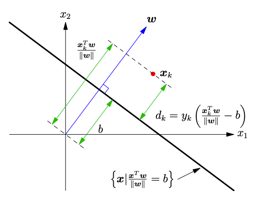
The black line in Figure 1 represents a hyperplane defined by an orthogonal vector $w$ and a bias $b$
$$ w^Tx - b||w|| = 0 $$
The distance from the origin to the hyperplane is given by
$$ \frac{w^Tx_0}{||w||} = \frac{ b||w||}{||w||} = b $$
Thus, the distance from a point $x_i$ ($x_i \neq 0$) to the hyperplane is given by
$$ d_i = \frac{w^Tx_i}{||w||} - b $$
Primal Problem
Our goal is to find $w$ and $b$ to maximise $\Delta$ subject to the following constraints
$$ y_i ( \frac{w^Tx_i}{||w||} - b) \ge \Delta \text{ for all i = 1, 2, 3, …, n} $$
Divide both sides by $\Delta$,
$$ y_i(\frac{w^Tx_i}{||w||\Delta} - \frac{b}{\Delta}) \ge 1 $$
Then define $w' = w/(||w||\Delta)$ and $b'= b/\Delta$,
$$ y_i(w'^Tx_i - b') \ge 1 $$
Note
$$ ||w'|| = ||\frac{w}{||w||\Delta}|| = \frac{1}{\Delta} $$
Therefore, minimising $||w'||^2$ is equivalent to maximising the margin $\Delta$. Now the problem becomes a quadratic programming problem defined below,
$$ \text{min}_{(w',b')} \frac{||w'||^2}{2} \text{ }\text{ }\text{ subject to $y_i(w'^Tx_i - b') \ge 1$ for all data points} $$
Extended Feature Space
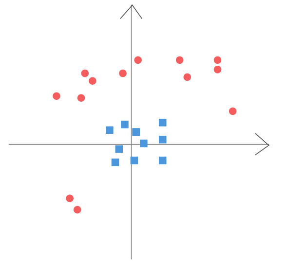
However, data are not always linearly separated, such as data in Figure 2.

Maybe we could do some data transformation and work in a new feature space where data are linearly speparable. Yea, in fact, SVM maps all feature vectors to an extended feature space by defining a special $\phi(x)$, which is a function of $x$
$$ x \rarr \phi(x) $$
Below are some examples of $\phi(x)$. You can choose any mapping you like.
$$ \phi(x) = x_1^2, \phi(x) = x_2^2, \phi(x) = \sqrt {x_1x_2} $$
Dual Form
In the extended feature space, we substitute $x$ for $\phi(x)$. So the question is defined as follows,
$$ \text{min}_{(w,b)} \frac{||w||^2}{2} \text{ }\text{ }\text{ subject to $y_i(w^T \phi(x_i) - b) \ge 1$ for all data points} $$
As mentioned earlier, we can use Lagrange multiplier to solve constrained optimisation. The Lagrangian function or the primal problem is given by
$$ \text{min}_{w, b}\text{max}_{\alpha} \mathcal{L} (w, b, \alpha) $$ where
$$ \mathcal{L} (w, b, \alpha) = \frac{||w||^2}{2} - \sum_{i=1}^N \alpha_i (y_i(w^T \phi(x_i) - b) - 1) $$
subject to $\alpha_i \ge 0$ (because we have inequality constraints).
Then we tranform the primal problem into the dual problem. We first minimise Lagrange function w.r.t $w, b$ then maximise with respect to $\alpha$
$$ \text{max}_{\alpha} \text{min}_{w, b} \mathcal{L} (w, b, \alpha) $$
Taking the derivative of $\mathcal{L} (w, b, \alpha)$ w.r.t. $w, b$ respectively,
$$ \nabla_w \mathcal{L} = w - \sum_{i=1}^N \alpha_i y_i\phi(x_i) = 0 $$
$$ \nabla_b \mathcal{L} = \sum_{i=1}^N \alpha_i y_i = 0 $$
Substituing back to the Lagrangian function
$$ \text{max}_{\alpha} \frac{||w||^2}{2} - \sum_{i=1}^N \alpha_i (y_i(w^T \phi(x_i) - b) - 1) $$
$$ = \text{max}_{\alpha} \frac{1}{2} \sum_{i=1}^N \alpha_i y_i\phi(x_i)^T \sum_{i=1}^N \alpha_i y_i\phi(x_i) - \sum_{i=1}^N (\alpha_i y_iw^T \phi(x_i) - \alpha_i y_ib - \alpha_i) $$
$$ = \text{max}_{\alpha} \frac{1}{2} \sum_{i=1}^N \alpha_i y_i\phi(x_i)^T \sum_{i=1}^N \alpha_i y_i\phi(x_i) - \sum_{i=1}^N (\alpha_i y_i (\sum_{j=1}^N \alpha_j y_j\phi(x_j)^T) \phi(x_i) - \alpha_i) $$
$$ = \text{max}_{\alpha} \frac{1}{2} \sum_{i=1}^N \alpha_i y_i\phi(x_i)^T \sum_{i=1}^N \alpha_i y_i\phi(x_i) - \sum_{i=1}^N \alpha_i y_i\phi(x_i)^T \sum_{j=1}^N \alpha_j y_j \phi(x_j) + \sum_{i=1}^N \alpha_i $$
$$ = \text{max}_{\alpha} \sum_{i=1}^N \alpha_i - \frac{1}{2} \sum_{i=1}^N \alpha_i y_i\phi(x_i)^T \sum_{j=1}^N \alpha_j y_j \phi(x_j) $$
$$ = \text{max}_{\alpha} \sum_{i=1}^N \alpha_i - \frac{1}{2} \sum_{i=1}^N \sum_{j=1}^N \alpha_i \alpha_j y_i y_j \phi(x_i)^T \phi(x_j) $$
The dual problem is to find $\alpha$ that maximise $\mathcal{L}$, subject to constraints
$$ \sum_{i=1}^N \alpha_i y_i = 0 $$
The Hessian of $\mathcal{L}$ is $-\frac{1}{2} X^TX$ where $X _{ik}$= $y_k \phi_i(x_k)$, so it’s negative seim-definite, and thus there is a unique maximum.
Soft Margin
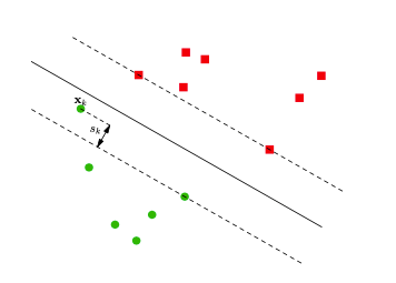
Okay, let’s just leave the dual problem alone for a while(we will go back in the next section). Now we look at another situation where we want to relax the margin constraints. In other words, we allow some samples to appear in the margin area. This is called soft margin. We do it by introducing a slack variable $s_i$ shown in Figure 3.

Now the constraint is
$$ y_i(w'^Tx_i - b') \ge 1 - s_i $$
where $s_k \ge 0$. Obviously, the value of $s_i$ includes three situations
- For samples that lies far away from the hyperplane, $s_i = 0$, because they are far enough
- For $0 \lt s_i \le 1$, there exist some samples that lie between margin and on the correct side of hyperplane
- For $s_i \gt 1$, samples are misclassified
Objective
The objective function becomes
$$ \text{min}_{(w',b')} \frac{||w'||^2}{2} + C\sum_{i=1}^N s_i $$
where $C$ controls the degree of misclassification we desire
- a small C allows more freedom to relax the margin, which means it’s acceptable to tolerate some misclassifications
- a large C means we want to correctly classify as many samples as possbile
The Lagragian function with slack variables is
$$ \mathcal{L} = \frac{||w||^2}{2} + C\sum_{i=1}^N s_i - \sum_{i=1}^N \alpha_i (y_i(w^T \phi(x_i) - b) - 1 + s_i) - \sum_{i=1}^N \beta_is_i $$
where $\beta_i$ are Lagrange multipliers that satisfy $\beta_i \ge 0$ (KKT condition)
Again, we minimise $\mathcal{L}$ w.r.t $s_i$
$$ \frac{\partial \mathcal{L}}{\partial s_i} = C - \alpha_i - \beta_i = 0 $$ So we have
$$ \alpha_i = C - \beta_i $$
Since $\beta_i \ge 0$,
$$ 0 \le \alpha_i \le C $$
Hinge Loss
By the way, the objective function can also be written in the following form
$$ \text{min}_{(w',b')} \frac{||w'||^2}{2} + C\sum_{i=1}^N \text{max} (0, 1-y_i f(x_i)) $$
where the second term is hinge loss function. So,
- $y_i f(x_i) \gt 1 $,
- $x_i$ is outside margin and on the right side of the hyperplane, so there is no contribution to loss
- $y_i f(x_i) = 1 $,
- $x_i$ is on the margin. Again, there is no contribution to loss
- $y_i f(x_i) \lt 1 $
- $x_i$ lies between the margin or it’s misclassified, so it increases the loss
Kernel Trick
Kernel
Kernel is simply the inner product in feature space,
$$ K(x, y) = \phi(x)^T \phi(y) = K(y, x) $$
where
- $\phi(x) = [\phi_1(x), \phi_2(x), …, \phi_k(x)]$
- $\phi_i(x)$ are real valued functions of $x$ ( $\phi_i(x)$ is just a real number )
- $k$ is the number of $\phi_i(x)$; it could be a specific number or INFINITE( that’s crazy! )
so kernel tells us the closeness or similarity between $x$ and $y$. The space spanned by $\phi(x)$ is called feature space or kernel space
$$ \mathcal{K} = \text{span } [ \phi(x) | x \in \mathcal{X} ] \in R^k $$
Symmetric
Given a kernel $K: \mathcal{X} \times \mathcal{X} \rarr R$ and a training data set $\mathcal{X} = [x_1, x_2, …, x_n]$, we can construct a kernel matrix or Gram matrix $G \in R^{n \times n}$
$$ G_{ij} = K(x_i, x_j) $$
Obviously, $G$ is a symmetric matrix and can be decomposed into $G = X^TX$, where
- $X$ is a $k \times n$ matrix
- each column of $X$ is $\phi(x_i)$
Positive Semi-Definite
Consider a new vector $w = X v \in R^k$, we have
$$ ||w||^2 = v^TX^T Xv = v^TGv \ge 0 $$
Hence, $G$ is positive semi-definite and all eigenvalues of $G$ are equal or greater than zero, i.e. $\lambda_i \ge 0$.
Eigenfunction
Remember the eigenvector of $G$ is defined as follows
$$ Gv = \lambda v $$
This means,
$$ \sum_{j=1}^n G_{ij} v_j = \lambda v_i $$
If we extend the dimention of $G$ to INFINITE, as shown in Figure 4, we have
$$ \sum_{j=1}^{\infin} G_{ij} v_j = \sum_{j=1}^{\infin} K(x_i, x_j) v_j = \lambda v_i $$
![Figure 4: G could have infinite dimension (Ref[3])](/blog/post/images/kernel-infinite.png)
Then we define an eigenfunciton $\psi(x)$, which is a real funtion of $x$
$$ \sum_{j=1}^{\infin} K(x_i, x_j) \psi(x_j) = \lambda \psi(x_i) $$
With the help of the integral operator, we can rewrite it as follows,
$$ \int_{y \in \mathcal{X}} K(x, y) \psi(y) dy = \lambda \psi(x) $$
Thus, $Gv = \lambda v$ is just a special case of this, when $\mathcal{X}$ is a finite set.
Mercer’s theorem
In general there will be a denumerable set of eigenfunctions $[ \psi_1(x),\psi_2(x), … ] $ and the corresponding $[\lambda_1, \lambda_2, …]$ where
$$ K(x, y) = \sum_i^{\infin} \lambda_i \psi_i(x) \psi_i(y) $$
This is known as Mercer’s theorem. And we find that $G_{ij} = \sum_{k=1}^n \lambda v_i^k v_j^k$ is just a special case of this, when $\mathcal{X}$ is a finite set.
If we define $\phi_i(x) = \sqrt \lambda_i \psi_i(x) $ then
$$ K(x, y) = \sum_i^{\infin} \sqrt \lambda_i \psi_i(x) \sqrt \lambda_i\psi_i(y) = \sum_i \phi_i(x) \phi_i(y) = \phi(x)^T \phi(y) $$
An immediate consequence is that for any real $\psi(x)$,
$$ \int_{x \in \mathcal{X}} \int_{y \in \mathcal{X}} K(x, y) \psi(y) \psi(x) dy dx $$
$$ = \int_{x \in \mathcal{X}} \int_{y \in \mathcal{X}} (\sum_i^{\infin} \lambda_i \psi_i(x) \psi_i(y)) \psi(y) \psi(x) dy dx $$
$$ = \sum_i^{\infin} \int_{x \in \mathcal{X}} \int_{y \in \mathcal{X}} [\sqrt\lambda_i \psi_i(y) \psi(y)] [\sqrt\lambda_i \psi_i(x) \psi(x) ] dydx $$
$$ = \sum_i^{\infin} \int_{x \in \mathcal{X}}[\sqrt\lambda_i \psi_i(x) \psi(x) ] (\int_{y \in \mathcal{X}} [\sqrt\lambda_i \psi_i(y) \psi(y)] dy) dx $$
$$ = \sum_i^{\infin} (\int_{x \in \mathcal{X}}[\sqrt\lambda_i \psi_i(x) \psi(x) ] dx)^2 \ge 0 $$
Thus, $v^TGv \ge 0$ is just a special case of this, when $\mathcal{X}$ is a finite set.
Putting it together, the following statements are equivalent,
-
$K(x, y)$ is positive semi-definite
-
The eigenvalue of $K(x, y)$ are non-negative
-
The kernel can be written $$ K(x, y) = \sum_i^{\infin} \lambda_i \psi_i(x) \psi_i(y) = \sum_i \phi_i(x) \phi_i(y) $$ where $\phi(x)$ are real functions
-
For any real function $\psi(x)$ $$ \int_{x \in \mathcal{X}} \int_{y \in \mathcal{X}} K(x, y) \psi(y) \psi(x) dy dx \ge 0 $$
Properties of Kernels
Adding Kernels
If $K_1(x, y)$ and $K_2(x, y)$ are valid kernels then $K_3(x, y) = K_1(x, y) + K_2(x, y)$ is also a kernel
$$ \int_{x \in \mathcal{X}} \int_{y \in \mathcal{X}} K_3(x, y) \psi(y) \psi(x) dy dx $$
$$ = \int_{x \in \mathcal{X}} \int_{y \in \mathcal{X}} (K_1(x, y) + K_2(x, y)) \psi(y) \psi(x) dy dx \ge 0 $$
Similarly, If $K(x, y)$ is a valid kernel so is $cK(x, y)$ for $c \gt 0$.
Product of Kernels
If $K_1(x, y)$ and $K_2(x, y)$ are valid kernels then $K_3(x, y) = K_1(x, y) K_2(x, y)$ is also a kernel
$$ K_3(x, y) = K_1(x, y) K_2(x, y) = \sum_i \phi_i^1(x) \phi_i^1(y) \sum_j \phi_j^2(x) \phi_j^2(y) $$
$$ = \sum_i \sum_j \phi_i^1(x) \phi_j^2(x) \phi_i^1(y) \phi_j^2(y) $$
Define $\phi_k(z) = \phi_i^1(z)\phi_j^2(z)$, and the number of $\phi_k(z)$ is $i * j$
$$ K_3(x, y) = \sum_k \phi_k(x) \phi_k(y) $$
Exponentiating Kernels
$\text{exp} (K(x, y))$ is a valid kernel since
$$ exp(K) = 1 + K + \frac{1}{2} K^2 + … $$
since the addition and multiplication of kernels yield valid kernels, each term is also a kernel and therefore the exponential of a kernel is a kernel.
Common Kernels
TODO
Linear
Gaussian
Quadratic
Comments
- SVM relys on distances between data points, so it would be better to normalise data if we don’t know what features are important.
- Different C can make a great difference in performance. We can use cross-validation to choose the optimal C.
- A linear decision boundary doesn’t always exist, especially we obtain a poor performance. If so, we might try a non-linear boundary with Kernel. There are many kernel functions designed for particular data types. Often, Kernel comes with its parameters, so fine-tunining them is also important to improve model’s performance.
- We don’t need to explicitly know what $\phi(x)$ are. All we need to know is that there exist a hyperplane that can separate the data linearly in a higher dimensional space. Though we are in the extended feature space, we do computation of the inner product in the original feature space.
References
[2] http://crsouza.com/2010/03/17/kernel-functions-for-machine-learning-applications/
[3] https://www.cs.cmu.edu/~bapoczos/other_presentations/kernel_methods_01_10_2009.pdf